2008 – Page 15 – The Sport Journal

Do Reliable Predictors Exist for the Outcomes of NASCAR Races?

Submitted by: C. Barry Pfitzner & Tracy D. Rishel

Introduction

This research attempts to ascertain whether factors known prior to a NASCAR race can help to predict the order of finish of that race. We provide evidence in the form of correlation analysis of the order of finish with available quantitative and categorical information collected, and a simple test for the effect of teams (regressions for each races are also available from the authors). Data were collected on 14 races from the 2003 NASCAR Winston Cup (now Nextel Cup Series) schedule.

Many factors influence the outcomes of NASCAR races. The speed and handling of the car, the skill of the driver, and the performance of the pit crew are but a few of the variables that are important determinants of the finish for a particular car and driver. Many variables outside the control of a particular team, such as the behavior of other drivers, weather, cautions, and the like also influence the final order of finish in NASCAR races. A priori, then, it would be anticipated that predicting outcomes in any meaningful way would be problematical.

The goal of this project is to determine whether those objective, measurable, variables known prior to the start of a race are useful in determining the order of the outcome. To this end we have assembled full data sets for 14 different races from the 2003 NASCAR Winston Cup series. The data include the following for each race: the order of finish, pole position, qualifying speed, practice time, the number of team members of a given driver in the race, the finish position in the prior race at that particular venue, the finish position in the immediately preceding race, driver points for the previous year in Winston Cup competition, and laps completed for the previous year in Winston Cup competition. We also have dummy variables to indicate whether it is the rookie year for a driver and whether the driver changed teams for the current year.

A Simple Model

As a first approach to the problem of predicting the order of finish in particular NASCAR races, we offer a simple theoretical model. Order of finish is posited to be functionally related to variable sets reflecting car speed, driver characteristics, team characteristics, performance in related races, and other factors. In functional notation,

F = f(S, D, T, RR, O), where:

F = Order of finish for a particular race

S = Car speed

D = Driver characteristics

T = Team characteristics

RR = Performance in related races

O = Other factors

To be sure, the variable categories listed are not distinct from each other. That is, empirical measures of car speed are certainly related to other categories of variables such as driver and team characteristics. The theoretical model serves to provide a framework for the empirical specification of the model.

Car Speed, Driver Characteristics, and Related Races

The effects of car speed on race outcomes are obvious. Faster cars will, on average, finish better. Also obvious are the effects of driver racing skill and experience. If it is possible to proxy for driver racing skill and experience, such proxies should be related to finish position across races.

Car/driver combinations may also be subject to streakiness in consecutive races and they may also be more successful at particular venues. The empirical variables defined in the following section proxy for these effects.

Team Characteristics

Team characteristics, in particular team size, require additional explanation. It is an empirical fact that multi-car teams have, in recent years, dominated the NASCAR Winston Cup series, and it is commonly believed that multi-car teams have advantages over smaller teams. What particular advantages are possible for multi-car teams?

First, the marginal cost of increasing the speed of a car is likely to be very sharply upward sloping (Allmen, 2001). This is due in part to NASCAR rules regarding car shape, size, aerodynamics, weight, and engine characteristics. While these rules are in place to equalize competition, the existence of this degree of uniformity makes it very difficult and expensive to gain an advantage within the rules. As Bill Elliott, a driver and past owner observes, “It may cost you $5 million to get to the track, but it may cost you an additional $3 million for a few tenths better lap time ….” (Middleton, 2000, p. 37).

A team with more car/driver combinations can apply any found advantage to each of its cars. Such advantages then result in better performances for all cars on the team, and hence greater performance revenues. Consider Figure 1 in which marginal cost (MC) increases sharply as car speed increases and such costs are assumed to be the same for multi-car teams as for single car teams. Since newly discovered speed advantages can be applied to all cars on a multi-car team, those teams can generate greater revenues for the team (MR M = marginal revenue for multi-car teams) than any such advantage generates for a single car team (MR S = marginal revenue for single car teams). Following optimization principles then, multi-car teams would find it worthwhile to achieve a speed of S M, whereas single car teams have incentive to achieve a speed of only S S. If this analysis is correct, multi-car teams would be expected to achieve greater speed in general than single car teams.

Second, it is an empirical fact that larger teams attract greater sponsorship resources, in part because they are more successful. Then, if the sharply increasing marginal costs mean that multi-car teams are more likely to engage in expensive research for given performance benefits and sponsorship revenues depend on performance, the dominance of multi-car teams can be explained (at least in part) by this simple economic analysis.

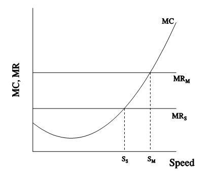
Figure 1: Multi-car versus single car teams

Third, teams with more sponsorship income are able to offer greater compensation to crewmembers, hire more experienced and specialized team members, such as aerodynamicists, and can more easily afford expensive technology and testing.

Fourth, substantial barriers to success for smaller teams (especially single car teams) may also exist because of scale economies. The advanced technology machinery for making racing parts would be an example of the “lumpy inputs” explanation of scale economies thought to be the most common reason for decreasing long run average cost. Larger teams would then have an advantage since the production of such parts for the team would necessarily be larger in scale.

Other advantages also accrue to multi-car teams. Operationally, multi-car teams also have more test dates available to them at Winston Cup tracks. Hence, more data can be collected and shared among team members when it comes to setting up the cars for races at those tracks. Multi-car teams also have built-in drafting partners, although the NASCAR literature suggests that at the end of the race each driver is “on his own,” (Cotter, 1999; Dolack, 2003; Hinton, 1997; Pearce, 1996, 2003).

Empirical Specification: Races and Data

The data for this project were collected from a variety of Web sites, http://www.nascar.com (Past Race Archive, 2002, 2003), http://jayski.thatsracin.com/ index.html (Statistics Pages from Jayski. 2002), and http://www.foxsports.com/named/ FS/Auto (Nextel Cup Standings, 2002, 2003). The variable we wish to predict is the order of finish, which is of course, available for each race on the Winston Cup circuit.

Individual Races

The 14 races for which we collected data include short tracks, speedways, super speedways, and a road course. To determine if the same factors are related to order of finish of different races at the same track, we also included both races run at Daytona and both races run at Michigan in 2003. The specific races for which we collected data are: the Brickyard 400 at Indianapolis Motor Speedway, the Food City 500 at Bristol Motor Speedway, the Coca-Cola 600 at Lowe’s Motor Speedway, the Carolina Dodge Dealers 400 at Darlington Raceway, the Daytona 500 at Daytona International Speedway, the Pepsi 400 at Daytona International Speedway, the Virginia 500 at Martinsville Speedway, the Sirius 400 at Michigan International Speedway, the GFS Marketplace 400 at Michigan International Speedway, the Chevy Rock & Roll 400 at Richmond International Speedway, the Aaron’s 499 at Talladega Superspeedway, the Samsung/Radio Shack 500 at Texas Motor Speedway, the Tropicana 400 at Chicagoland Speedway, and the Sirius at the Glen at Watkins Glen International.

The potential explanatory variables for order of finish collected for each race were as follows:

ptime = the practice time closest to race time.

qspeed = the speed at which the car/driver qualified.

pole = position of the car at the start of the race.

points = points scored in the Winston Cup Series for the prior year.

laps = number of laps completed for all Winston Cup races in the prior year.

DNF = did not finish, the number of races in which the driver failed to finish, prior year.

rookie = a dummy variable equal to 1 if the driver was a rookie in 2003, and equal to

0 otherwise.

# drivers = the number of cars/drivers a multi-car owner fields (for 2003, values = 1,2,3,4).

newteam = a dummy variable equal to 1 if the driver was a member of a new team in 2003, and equal to 0 otherwise.

prev = the finish position of the driver in the previous week’s race.

lastyr = the finish position of the driver in the 2002 running of the same race.

Car Speed

The first three variables from the above list, practice time, qualifying speed, and pole position correspond to the car speed category from the model outlined in the previous section. Clearly qualifying speed and pole position are very closely related (since pole position is determined primarily by qualifying speed), however race officials, for reasons such as a rule and/or equipment violation, missing the driver’s meeting, switching to a backup car, an engine change, or a driver change, may alter pole position. For this reason we collected data for both qualifying speed and pole position in case one or the other is a better predictor of race outcomes.

Driver Characteristics

The next four variables, points, laps, DNFs, and rookie, are driver characteristics with the first three representing performance in the prior year, and the variable rookie is a proxy for lack of experience on the Winston Cup circuit. Theoretically, rookies will not have the skill level that existing Winston Cup drivers have developed over the years, nor will they have had exposure to certain tracks that more experienced Winston Cup drivers have competed on in the past.

Team Characteristics

The variables # drivers and newteam correspond to the team characteristics category in the model. The # drivers variable measures the effect of a given owner having multiple cars/drivers or a multi-car team. With respect to the new team variable (newteam), drivers joining a new team will require time to adjust to the way the crew operates, in addition to developing an effective communication style with the crew chief.

Related Race Effects

Related race effects are measured by the variables prev and lastyr. The variable prev is an attempt to proxy for possible streakiness from race to race. That is, are good finishes followed by other good finishes and poor performances followed by poor performance in the following race? The variable lastyr attempts to measure whether a certain racetrack is a better venue for certain car/driver combinations. For example, the dominance of Dale Earnhardt, Incorporated (DEI) at the superspeedways illustrates the expertise a team may develop at specific racing venues (McCarter, 2002). Since 2001, DEI has won 9 out of the 12 races at Daytona International Speedway and Talladega Superspeedway.

Methodology and Expectations

As a first attempt to determine those variables that relate to order of finish, correlation coefficients are computed between order of finish and each of the measured explanatory variables. The following signs are anticipated for the correlation coefficients:

Expected Sign

of coefficient Explanation

Faster (lower) practice time leads to better finish

Higher qualify in speed (MPH) leads to better finish

Better pole position leads to a better finish

More points from previous year leads to a better finish

More laps completed from previous year leads to better finish

More failures to finish leads to poorer finish

Rookies may be less likely to have better finishes

Multi-car teams may have better finishes

Driver on new teams less likely to have better finishes

Previous race finish positively related to current race finish

Previous finish at this track positively related to current finish

Note: ρ represents the population correlation coefficient, and f represents finish position, 1 = winner , 2 = second place, etc..

Results

Correlation Analysis

Table 1 in the appendix is the result of the correlation computations. The coefficients in bold are statistically significant at the α = .05 level and consistent with the predicted signs presented in the previous section.

Several results of this exercise are interesting and potentially important for predicting the outcome of NASCAR races. First, considering the columns (how the variables fared across different races), on average the signs of the variables are in accord with expectations (though some are on the whole insignificant). Several of the variables seem to be consistently correlated (linearly) with order of finish across races. For example the number of drivers variable (# drivers) is statistically significant for all races except Darlington and Watkins Glen (even then the coefficients have the predicted sign). Of course that teams with more members tend to be more successful is not a new conclusion—these results support statistically, at the individual race level, the hypothesis that multi-car teams are generally more successful (see the section on team characteristics above). Of the two tracks that did not have statistically significant results with respect to the # drivers variable, the Watkins Glen result might be due to the fact that it is a road race. Watkins Glen is one of only two road courses utilized by Winston Cup, and teams often use substitute drivers with more road racing skills than their full-time driver may possess in these races.

Indicators of drivers’ past successes also are correlated with order of finish. The variable points is statistically significant for 11 of the 14 races and all of these sample correlations have the anticipated sign. Interestingly enough, the three races that did not demonstrate significant results were run at Daytona and Talladega, the two restrictor plate tracks. Similarly laps, which might be interpreted as a measure of driver/car consistency and driver experience, is statistically significant in 7 of the 14 races. The DNF variable seems to explain little in the way of simple correlation with order of finish. In considering this variable, recognize that a driver with more DNFs may have simply competed in more races than another driver. Thus simple correlation, which does not control for levels of other variables, may not be appropriate to measure such effects.

Measures that account for car/driver speed include pole position (pole), qualifying speed (qspeed) and practice time (ptime). We recognize that pole position and qualifying speed generally measure the same effect. Both are included here to see if one or the other is more closely correlated with order of finish. Based on the sample correlations in Table 1, qspeed is significantly related to order of finish in half of the races and pole in 6 of the 14 races. Practice time (ptime) seems to fare somewhat better—it is significantly related to order of finish in 9 of the 14 races. There may be several reasons for this outcome. The practice times used for statistical analysis were collected from the practice session conducted closest to race time, if all drivers participated in that session. If all drivers did not participate in the last practice session, then practice time statistics were taken from the session run closest to race time in which all drivers practiced. This was done to ensure that the cars would be “set up” in practice as close to race set-up as possible. Since the cars are set-up for race conditions when they practice, it would be expected that the ptime would more closely relate to order of finish than qspeed because the set-up for qualifying is based on two laps at the fastest speed possible. Race day set-up is designed to accommodate consistency and longer runs on the track.

The variable that measures the finish position in the driver’s last race (prev) is statistically related to order of finish in 8 of the 14 races and has the expected sign for all races. This would suggest that driver/car combinations are subject to streakiness, that is, good finishes tend to be followed by other good finishes and vice versa. For only four races is the variable lastyr, the finish position of the driver in the prior running of the race by the same name correlated with the current finish position.

Of the two categorical variables, newteam (equals 1 if the driver joined a new race team for the 2003 season, 0 otherwise) is related to order of finish in 10 of the 14 races and in all races has the anticipated sign. Changing teams, on average, would seem to be related to poorer finishes. On the other hand, rookie status (rookie) was related to finish order only for the first Daytona race and Martinsville.

Again considering the columns in Table 1, the average of the correlation coefficients for each of the explanatory variables across the 14 races is included in the table as the bottom row. A coefficient above 0.25 is generally statistically significant for individual races (again α = .05, one-tailed test, n = 43) On that basis, eight of the variables (laps, points, newteam, pole, # drivers, prev, ptime, and qspeed) are on average statistically (linearly) related to order of finish.

It is also useful to consider the correlations for individual races, i.e., to consider Table 1 by row. For example, at Martinsville order of finish was linearly related to 9 of the 11 variables in the explanatory variable set. The first (June) Michigan race, Richmond, and Chicagoland were linearly related to eight of the explanatory variables. At the other end of the scale, for the two Daytona races, only two of the explanatory variables were correlated with order of finish. One of those variables was the same (# drivers) for both Daytona races. Interestingly, comparing the second (August) Michigan race to the first, only five variables were statistically significant for the second race, but each of those variables was also significant for the first Michigan race. However, relatively strong correlations for pole, practice time and qualifying speed for the first Michigan race were not repeated for the second Michigan race. The reader may examine Table 1 to see that the rest of the races have from three to seven explanatory variables that are statistically significant.

Additional Evidence on Team Effect

The effect of team membership (#drivers) seems to play an increasingly important role in NASCAR (Cotter, 1999; Dolack, 2003; Hinton, 1997; Pearce, 1996, 2003). In 2003, 12 organizations owned and fielded 33 of the 43 cars competing at the majority of NASCAR races. Additionally the Winston Cup Championship has been won by a multi-car team in each of the last 10 years (Pearce, 2003). Therefore, we considered another test of team membership on car/driver success. Using statistics from the entire 2002 and 2003 racing years, a table of results divided into top 10 finishes and finishes out of the top 10 and classified by number of team members was constructed. Table 2 in the appendix shows that teams with four members (the highest number of team members at the start of 2002) had 285 starts and of those, 43.16% resulted in top 10 finishes. The corresponding percentages are 15.55% for three member teams, 29.14% for two member teams, and only 8.68% for drivers without team members. The largest (four member) teams tended to dominate the top 10 finishes. Perhaps surprising is the fact that two member teams had by far the largest number of starts and the second highest rate of top 10 finishes with 29.14%. For three member teams the corresponding percentage was 15.55% and single drivers finished in the top 10 only 8.68% of the time. A simple chi-squared test of independence of the classification of top 10s by number of drivers on a team, yields a χ 2 = 123.9, which allows rejection of the null of independence at α < 0.001. This result confirms the obvious result that the proportion of top 10 finishes does depend on the number of team members.

Table 3 contains the same categories for the 2003 Winston Cup drivers. There was one team with five drivers for the 2003 season, so the table contains an additional column. For the 2003 season, the percentage of top 10 finishes is remarkably constant for the teams with five, four and two members, with 37%, 38% and 32% respectively. Again, teams with three members and especially the single drivers fared less well on the basis of top 10 finishes. Again, the null hypothesis of independence between number of team members and top 10 finishes can be rejected (χ 2 = 106.0), providing statistical confirmation of the already clear evidence that the proportion of top 10 finishes differs by number of team members.

Conclusions

The correlation analysis across 14 races for the 2003 NASCAR Winston Cup series identifies a number of variables that are associated with the order of finish of these races. On average, variables measuring car speed, including practice time, qualifying speed, and pole position are related to the order of finish of races. We also find that prior success on the part of the driver, measured by laps completed in the prior year and points accumulated are also correlated with order of finish. Whether or not the driver was a rookie was, perhaps surprisingly, not on average correlated with finish order across races. There is also some evidence that performances of driver/car combinations are subject to streaks. That is, finish positions in a given race are often correlated with finish positions in the race that follows. Of course these results could simply reflect the fact that some driver/car combinations consistently finish better than others may. Changing teams is correlated with poorer finishes and team size is correlated with better finishes.

The effect of team membership is reinforced by the data in Tables 2 and 3, which classifies top 10 finishes by number of team members. Teams with more members are more successful in terms of top 10 finishes. However, this effect is not monotonic in nature, since two member teams have a larger percentage of top 10s than do teams with three members.

Further research is indicated to test the robustness of these results. Such analysis could include races not in our data set and results from different years of NASCAR racing.

References

Allmen, P. von. (2001). Is the reward system in NASCAR efficient? Journal of Sports Performance, 2(1), 62-79.

Cotter, T. (1999). Say goodbye to the single-car team. Road & Track, 50(8), 142-143.

Dolack, C. (2003). One is the loneliest number. Auto Racing Digest, 31(6), 66.

Hinton, E. (1997). Strength in numbers. Sport Illustrated, 87(16), 86-87.

McCarter, M. (2002). Stepping up to the plate. The Sporting News, 226(27), 38-39.

Middleton, A. (2000, February). Racing’s biggest obstacle. Stock Car Racing, 34-37.

Past Race Archive, 2002 [Data files]. Available from NASCAR Web site, http://www.nascar.com

Past Race Archive, 2003 [Data files]. Available from NASCAR Web site, http://www.nascar.com

Nextel Cup Standings, 2002 [Data files]. Available from FOXSports Web site, http://www.foxsports.com/named/FS/Auto

Nextel Cup Standings, 2003 [Data files]. Available from FOXSports Web site, http://www.foxsports.com/named/FS/Auto

Parsons, K. (2002, August 26). Tunnel vision – NASCAR teams’ fortunes are blowing in the wind. The Commercial Appeal, Memphis, TN, p. D9.

Pearce, A. (1996). Fair and square. AutoWeek, 46(50), 40-41.

Pearce, A. (2003). Going it alone. AutoWeek, 53(14), 57-58.

Statistics Pages from Jayski. (2002) [Data files]. Available from Jayski Web site, http://jayski.thatsracin.com/index.html

Appendix

Table 1: Correlation coefficients between finish position and the explanatory variables

Explanatory Variables

Race	Laps	DNF	Points	newteam	Pole	#drivers	prev	lastyr	ptime	qspeed	Rookie?
Indianapolis	-0.214	0.091	-0.319	0.342	-0.106	-0.326	0.118	0.435	0.374	0.047	0.088
Bristol	-0.209	0.316	-0.350	0.030	0.177	-0.417	0.117	0.407	0.392	-0.190	0.088
Lowe’s	-0.209	0.030	-0.291	0.360	0.198	-0.314	0.335	0.085	0.403	-0.283	0.200
Darlington	-0.373	0.154	-0.428	0.180	0.176	-0.153	0.170	-0.141	-0.239	-0.234	0.265
Daytona (Feb)	-0.044	-0.111	-0.173	0.155	0.243	-0.300	0.274	0.045	-0.106	NA	0.094
Daytona (July)	-0.140	0.110	-0.218	0.132	0.006	-0.258	0.167	0.300	0.164	-0.060	0.105
Martinsville	-0.462	0.079	-0.540	0.030	0.433	-0.342	0.314	0.352	0.462	-0.496	0.263
Michigan (June)	-0.383	0.115	-0.435	0.396	0.596	-0.550	0.478	0.125	0.549	-0.547	0.041
Michigan (Aug)	-0.342	-0.297	-0.408	0.380	0.172	-0.356	0.392	0.087	0.237	-0.205	0.212
Richmond	-0.367	-0.070	-0.508	0.384	0.406	-0.283	0.300	0.126	0.350	-0.403	0.228
Talladega	-0.228	0.088	-0.230	0.306	0.398	-0.335	0.098	0.233	0.080	-0.361	0.170
Texas	-0.200	0.085	-0.352	0.282	0.169	-0.393	0.195	-0.178	0.300	-0.159	0.146
Chicagoland	-0.339	0.064	-0.413	0.260	0.422	-0.261	0.317	0.246	0.428	-0.464	0.178
Watkins Glen	-0.410	-0.298	-0.472	0.406	0.297	-0.244	0.254	0.123	0.285	-0.278	0.239

Average	-0.280	0.025	-0.367	0.260	0.256	-0.324	0.252	0.160	0.263	-0.279	0.166

Table 2: Top Ten Finishes by Number of Team Members, 2002 Season

	4 member teams	3 member teams	2 member teams	One member teams
Top 10 %	43.16%	15.55%	29.14%	8.68%
Total starts	285	328	525	357

Table 3: Top Ten Finishes by Number of Team Members, 2003 Season

	5 member teams	4 member teams	3 member teams	2 member teams	One member teams
Top 10 %	36.87%	38.19%	22.53%	31.67%	7.66%
Total starts	179	144	395	360	418

The flat MR curves are offered as an approximation. Additional speed should add increasing marginal revenue (as cars move up in finish order, added revenue increases), but since all cars are attempting to increase speed, the possible increases in revenue will be distributed among the competitors.

For example, testing for the aerodynamic properties of a car in a wind tunnel can cost more than $2000 per hour (Parsons, 2002).

T he field is generally set using a combination of timed laps and provisionals. The fastest 36 cars earn a place based on time, while positions 37-43 are determined by a process which may include last season’s final owners standings, current owners standings and former champions. The provisionals are assigned in descending order, beginning with the highest ranking owner in the standings. The lone exception is the Daytona 500, which uses two qualifying races to determine the field. (Nascar.com)

In other words, a driver with many laps completed and many DNFs would be expected to fare less well than another driver with many laps completed, but few DNFs.

While the sample size is generally 43 for individual races it is somewhat lower for some individual races, e.g., a race in which a driver/car combination did not run in the race at a particular venue it its previous iteration.

If all four members of a team start in the same race, that would equal 4 starts and if two of those four finish in the top 10, that would be 50% in the top 10.

This procedure can also be described as a test of proportions, that is, we have evidence that the proportions of top 10 finishes differs by number of team members.

U.S. Sports Academy2016-10-14T11:50:19-05:00March 4th, 2008|Contemporary Sports Issues, Sports Studies and Sports Psychology|Comments Off

The Olympic Odyssey

Submitted by: Dr. Thomas P. Rosandich – USSA President and CEO

Athens, Greece – I am starting the writing of this President’s Column from a small island in the Aegean Sea, an hour out of Athens, and am enjoying the magnificent villa home of Joe and Mina Valyraki. Joe has served in the Greek government for more than 25 years. He was the Minister of Sport when they signed the agreement to bring the Athens Olympiad 2004 to its original home in Greece. He then served twice as a Minister of the Interior – security is a specialty of his. His beautiful wife, Mina, was the Academy’s Sport Artist of the Year in 2002 (see picture above).

This is my first stop in a world sports tour to view Academy programs throughout the world. Currently, I am here as an observer of the Games. But this is far from my first visit to Athens as the Academy has had various projects in Greece in the past and several in the last eight years.

I feel like my travels are an ongoing “Odyssey” not unlike Homer’s tale of Odysseus after the Trojan War. Webster describes an odyssey as “a long wandering trek marked by many changes of fortune.”

My odyssey has been one of sport that has taken me to every Olympiad since Melbourne 1956, when I was a U.S. Marine Corps Officer and the All Service Coach. At that period of time, the majority of the athletes on the U.S. Track and Field Team were from the military because the draft was very much a part of life in America. Since then, during the past 50 years, I have had the privilege of visiting over 100 countries, and the Academy has developed sport programs in one form or another in more than half of them.

This has been an exciting Olympics in Greece. Each day, we have driven from Eretria on the island of Evia to take in a variety of Olympic events, e.g. water polo,

volleyball, and of course, track and field, the centerpiece of all Olympiads. (Incidentally, for anyone interested in what the original games were really all about, I recommend “The Naked Olympics” by Tony Perrottet).

I believe this to be the best Olympics I have seen in the last 48 years and probably the best in modern times. In many ways it was a miracle. I have been coming to Athens continuously over the last eight years, and I thought that Jacques Rogge, the President of the IOC, was correct when he almost took the Games away from the Greeks, fearing that they would not be ready. However, apparently if you tell the Greeks they can’t do something, they will go out and prove that they can indeed do it – and they did it in spades with these Games. I rate them A-plus – even better than the Seoul Olympics of 1988, which I thought was the best to date, except for the Korean language problem.

The Greeks made it all come together in the very end. I have never traveled so easily around Athens! Not long ago, it was nothing short of a nightmare just getting from Athens to their beautiful new airport. The underground trains were not useable except for small segments within the city, and many ring roads led to nowhere. But by magic, it all hooked up with the kind of “discipline” you usually only find in Asian cultures like Japan.

The ring roads around Athens cleared the gridlock, a trademark of the city. These roads were built with private money, which will be repaid through tolls in the coming years. This is a classic example of the private sector working with the government to achieve a common goal. Incidentally, all of these new roads lead from a beautifully built Olympic village, designed like a city – complete with shops, hospitals and all the normal city services; certainly one of the biggest and best ever built. The roads through the stadiums have a lane marked off with orange paint for Olympic vehicles only, and any violation of that policy carries a stiff $157 fine. A real coup by the Olympic committee is that, if you have an Olympic ticket, you can get on all public transport free of charge.

The Olympic complex, particularly the main stadium, is spectacular and architecturally brilliant, displaying the artistic hand of the Spanish architect, Santiago Clatrava. The stadium grounds are immaculate. They are set off by reflecting pools and a Spanish art piece, called the “WAVING WALL,” 100 meters long, that chimes throughout the night and serves as the backdrop for endless projected Olympic competitions, like a giant outdoor movie theater.

The grounds surrounding the sport complex are impeccable. At midnight, after a track and field event, I watched as 72,000 spectators (basically Greeks) carried their trash and bottles (from vendors like McDonald’s and Coca Cola – the major sponsors of the Games) and put them into the bins provided outside the stadium. Where else have you seen this?

A diverse group of some 65,000 volunteers, including the disabled in wheelchairs, was organized to help everyone and anyone attending the Games. It was one of the best-trained and most helpful “Corps of Volunteers” I have ever seen at a Games. Originally, the goal was for 45,000 volunteers but the foreign volunteers increased the total to some 65,000. All were dressed in an attractive common uniform, including some 15,000 “extras.” As spectators left the stadium and the Olympic grounds, dozens of well-groomed and cordial ladies called out from judges chairs “good night,” “goodbye,” “sweet dreams,” “travel safely” and other such hospitable farewells.

Before I leave the topic of the Olympic complex and the grounds, I would like to congratulate the Greeks on how they laid out and installed their shopping centers – again, some of the best that I have seen. Major sponsors paid millions to use the Olympic Rings and the remarkable thing was that there was no “ambush marketing.” The prices were standardized for all the Olympic clothing and mementos. They were the same whether they were sold on the Olympic grounds, in the city of Athens, or indeed on the outer islands. I particularly was aware of this as I shopped for family, staff and friends. Even more important, bottled water, for instance, was cheaper on the Olympic grounds than in the normal grocery store.

Unfortunately, this was a total reverse of what happened in Atlanta in 1996, where vendors were selling the same items at different prices five feet from each other down every side street. I rated the Atlanta Olympics as a C-minus, at best, as so did the rest of the world, I believe.

Throughout the streets of Athens there were continuous athletic and cultural programs late into the night for weeks, and there was a mass of well-behaved crowds. Again, this was not only throughout Athens but in the suburbs and on the outer islands, all well run without rowdy crowds.

What Athens did was rebuild itself for years to come. I call this the “Barcelona Model.” I watched Barcelona during the early 90’s and certainly during the Games, as it built new roads, airports, hotels, streets and apartments; while eliminating slums and the factory district, and recapturing the polluted Mediterranean, much like Sydney rebuilt itself in 2000. The only city that was not able to take the great opportunity of the Olympics to rebuild its inner structure was Atlanta. In fact, they ended up as probably the only Olympic city that lost their Olympic stadium, which in this case is now Turner’s Field for the Atlanta Braves baseball team.

I thought that Athens not only did a remarkable job of rebuilding itself but it did so without destroying its great antiquities, such as the Acropolis. (I, for one, hope the British give back the marble facings they took at the time of the Turkish occupation.)

Incidentally, I was in Barcelona earlier this year for Olympic meetings with the IOC Culture and Olympic Education Commission, on which I am privileged to serve. The reconstruction and the development of Barcelona that was done for the 1992 Olympic Games has not stopped. I hope that will be true with Athens.

Lastly, the greatest miracle of the Olympiad was the security. Guards and special electronic equipment were everywhere at an estimated cost of $1.6 billion. Security was everywhere, from helicopters above to cameras sliding on cable over every stadium, with checkpoints throughout the Olympic sites. It was subtle but with a touch of class. Such a touch of class is needed with our TSA people managing airport security throughout the USA.

The greatest problem in this Olympiad was drugs, as the Greeks lost some of their best sprinters at the beginning of the Games. Performance enhancing drugs could destroy the Games, along with violence and corruption.

There is no question that these were the best Games ever. It didn’t come cheap! The estimated cost was $12 billion – the most costly Games ever and a debt the Greek people will pay for generations. But from my perspective, the Greeks are prepared to do so.

In the Closing Ceremonies, Gianna Angelopaulos-Daskalaki, President of the Athens 2004 Organizing Committee, told of the achievements of the Greek people in bringing these Games together, which did in fact conclude once again with one of the most spectacular closing ceremonies that the world has ever seen. The opening ceremonies were equally spectacular. Rogge said at the end of the Games: “The Greek people have won!” and indeed they had!

Most importantly for us, after the Games, the Academy will have ongoing sport education programs in Greece with both the Greek Olympic Committee and some of the country’s better colleges and universities via distance learning.

I left Greece the following day for Cyprus, a Greek-speaking island nation some 45 minutes south of Greece by air. As we traveled to the airport everyone forgot the orange line on the highway, and we were back to driving like the Greek people of old. Some things will never change.

U.S. Sports Academy2013-11-26T19:27:43-06:00March 3rd, 2008|Contemporary Sports Issues, Sports Facilities, Sports Management|Comments Off

A Personal Odyssey to Greece and the 2004 Olympic Games

Submitted by: Scott J. Callan, Ph.D. & Janet M. Thomas, Ph.D.

Abstract

An extensive body of research examines the importance of a golfer’s
shot-making skills to the player’s overall performance, where performance
is measured as either tournament money winnings or average score per round
of golf. Independent of the performance measure, existing studies find
that a player’s shot-making skills contribute significantly to explaining
the variability in a golfer’s performance. To date, this research
has focused exclusively on the professional golfer. This study attempts
to extend the findings in the literature by examining the performance
determinants of amateur golfers. Using a sample of NCAA Division I male
golfers, various shot-making skills are analyzed and correlated with average
score per round of golf. Overall, the findings validate those dealing
with professional golfers. In particular, the results suggest that, like
professional golfers, amateurs must possess a variety of shot-making skills
to be successful. Moreover, relative to driving ability, putting skills
and reaching greens in regulation contribute more to explaining the variability
in a player’s success.

Introduction

Davidson and Templin (1986) present one of the first statistical investigations
of the major determinants of a professional golfer’s success. Using
U.S. Professional Golf Association (PGA) data, these researchers find
that a player’s shot-making skills explain approximately 86 percent
of the variability in a player’s average score and about 59 percent
of the variance in a player’s earnings. Based on these results,
Davidson and Templin conclude that a professional golfer must possess
a variety of shot-making skills to be successful as a tournament player.
They further offer strong empirical support that hitting greens in regulation
and putting were the two most important factors in explaining scoring
average variability across players, with driving ability showing up as
a distant third.

Following Davidson and Templin (1986), a number of researchers have
continued to investigate the determinants of a professional golfer’s
overall performance. Examples include Jones (1990), Shmanske (1992), Belkin,
Gansneder, Pickens, Rotella, and Striegel (1994), Wiseman, Chatterjee,
Wiseman, and Chatterjee (1994), Engelhardt (1995, 1997), Moy and Liaw
(1998), and more recently Nero (2001), Dorsel and Rotunda (2001), and
Engelhardt (2002). Overall, these studies support the major conclusion
presented by Davidson and Templin (1986), which is that a professional
golfer must exhibit a variety of shot-making skills to be successful as
a touring professional. While the relative importance of these skills
to player performance is not uniform across these studies, there is a
developing consensus that shot-making skills like putting and hitting
greens in regulation are more important to a player’s success than
driving distance.

Interestingly, while there is an accumulating literature investigating
professional golfers, no analogous studies have examined the amateur player,
despite the fact that Davidson and Templin (1986) explicitly state that
this avenue of investigation would be a useful direction for future research.
More recently, Belkin, et al. (1994) specifically raise this point, suggesting
that:

“It would also be intriguing to examine whether the same
skills which differentiate successful professionals also contribute
in the same manner to the fortunes of amateurs of differing capabilities.”
(p. 1280).

By way of response, this study fills that particular void in the literature
by empirically estimating the relationship between an amateur golfer’s
overall performance and various shot-making skills. To facilitate direct
comparisons to the existing literature on the determinants of professional
golfers’ performance, we employ the basic approach used by Davidson
and Templin (1986) and Belkin, et al. (1994), among others.

Method

Sample

The sample used for this analysis is a subset of NCAA Division I male
golfers who participated in at least one tournament during the 2002–2003
season. Table 1 presents a listing of the colleges and universities represented
in the study and the number of players from each institution. The specific
data on these collegiate golfers are obtained from Golfstat, Inc. (2003)
(accessible on the Internet at www.golfstat.com), and/or from the respective
colleges and universities directly. The colleges and universities included
in the analysis are a subset of the college teams participating in National
Collegiate Athletic Association (NCAA) Division I Men’s Golf. While
it would be preferable to examine all Division I teams, the individual
player statistics needed to perform the analysis are not available. However,
since it is reasonable to assume that the schools listed in Table 1 are
a representative sample of all Division I men’s teams, the data
sample is appropriate for this study.

TABLE 1
Sample of Schools Included in the Study

School	Number of Golfers	Conference	Golfweek/Sagarin Ranking
Clemson University	5	Atlantic Coast	1
University of Arizona	11	Pacific 10	7
University of Southern CA	9	Pacific 10	23
Duke University	8	Atlantic Coast	25
Vanderbilt University	7	Southeastern	31
California State -Fresno	9	Western Athletic	33
University of Kentucky	9	Southeastern	45
Georgia State University	8	Atlantic Sun	51
Texas A&M University	9	Big 12	60
Southeastern Louisiana Univ.	8	Southland	71
Coastal Carolina University	10	Big South	76

Sources: Golfstat, Inc. (2003) “Customized Team Pages-Men.”
www.golfstat.com/2003-2004/men/mstop10.htm, (accessed June 16, 2003),
various teams; Golfweek. (2003) “Golfweek/Sagarin Performance Index –
Men’s Team Ratings.” www.golfweek.com/college/mens1/teamrankings.asp,
(accessed July 1, 2003).

Measures

For the schools represented in this study, Golfstat, Inc. collects and
reports individual player statistics necessary to complete a performance
analysis. For this study we used statistics for the 2002 – 2003
NCAA Division I tournament season. Among the available data are the average
score per round (AS) for each amateur player in the sample. This statistic
provides the performance measure needed for the dependent variable in
this study, since earnings are not relevant to amateurs. Specifically,
according to the United States Golf Association (2003, p. 1) and the Royal
and Ancient Golf Club of St. Andrews (2003, p.1), an amateur golfer is
defined as:

“…one who plays the game as a non-remunerative and
non-profit-making sport and who does not receive remuneration for teaching
golf or for other activities because of golf skill or reputation, except
as provided in the Rules.”

Although studies of professional golfers examine scoring average and/or
earnings as performance measures, Wiseman et al. (1994) argue that correlation
results are stronger when scoring average is used. Hence, the use of scoring
average for this study of amateurs is soundly supported by the literature
examining professional golfers.

Statistics for the primary shot-making skills typically used in the
literature are collected and reported by Golfstat, Inc. and by some colleges
and universities. These include measures of driving accuracy, greens in
regulation, putting average, sand saves, and short game.

To capture amateurs’ long game skills, we use one of the classic
measures, which is driving accuracy. Specifically, we use the variable
Fairways Hit, which is defined as the percentage of fairways hit on par
4 and par 5 holes during a round of golf. Data on driving distance for
the amateur sample are not available. However, Dorsel and Rotunda (2001)
present evidence suggesting that the number of eagles (i.e., two strokes
under par on any hole) a player makes is positively correlated with the
player’s average driving distance. Hence, we use the variable Eagles,
the total number of eagles a player makes during the season, to control
for each player’s average driving distance. Following the literature,
we also include the variable Greens in Regulation (GIR) to measure the
percentage of greens a player reaches in regulation for the season. This
is defined as one stroke for a par three, two strokes or less for a par
four, and three strokes or less for a par five. As discussed in Belkin
et al. (1994), this GIR variable captures a player’s iron play and
their success at reading a green within the regulation number of strokes.

With regard to the short game, several variables are used in the analysis.
In keeping with the literature, we use two measures of putting skill –
Putts per Round, defined as the average number of putts per round, and
GIR Putts, which is the average number of putts measured only on greens
reached in regulation. Belkin, et al. (1994) is one study that uses the
former measure, while Dorsel and Rotunda (2001) is an example of a study
using the latter. Interestingly, Shmanske (1992) argues that the latter
statistic, GIR Putts, is superior because it correctly accounts for the
longer putting distances associated with a player who achieves a higher
number of greens in regulation. By including one of these measures in
different regression models, we can assess the validity of that argument.
We also include the variable Sand Saves (SS), which measures the percentage
of time a golfer makes par or better when hitting from a sand bunker.
In certain specifications of our regression analysis, we experiment with
the variable Short Game as an alternative measure to Sand Saves. Short
Game measures the percentage of time a player makes par or better when
not reaching the green in the regulation number of strokes.

In addition to a player’s shot-making skills, Belkin, et al. (1994)
and others note the importance of experience in determining a player’s
success. To control for this factor, two experience measures are used.
First, we define the variable Rounds as the number of tournament rounds
completed by each player during the 2002–2003 season. In a sense,
this measure captures a player’s short-term experience, in that
it measures how each additional round played in a season increases the
experience that a player can call upon in subsequent rounds. Second, to
control for longer-term cumulative experience, we construct a set of dummy
variables to reflect the player’s academic age, (i.e., Freshman,
Sophomore, Junior, or Senior). It is hypothesized that the higher a player’s
academic age, the more collegiate golfing experience has been gained,
and therefore the lower the expected average score.

Finally, since golf at the collegiate level is a team sport, it is important
to capture any associated team effects. That is, a player’s performance
might be affected by the team with which they are associated. At least
two plausible explanations for this team effect are viable – one
relating to the team’s coach and the other relating to the courses
played. With regard to the former, each team’s coach is expected
to uniquely affect the success of each team member through mentoring,
leadership, instruction, and overall direction. In fact, Dirks (2000)
and Giacobbi, Roper, Whitney, and Butryn (2002) present evidence supporting
the importance of a coach’s influence on the performance of a collegiate
athlete. Primarily, the coach acts as the team leader and instructor.
As a leader, the coach is responsible for the overall team strategy and
for ultimately determining a player’s tournament participation.
As an instructor, the more experienced coach may be better able to teach
players and to motivate them to improve their play.

As for courses played, we expect a player’s scoring average to
be affected by the specific golf courses played, which in turn are not
consistent across collegiate teams. Indeed, it is highly plausible that
some teams might, for example, play easier courses throughout a given
tournament season, which may lower a team member’s score. To account
for these team effects, dummy variables are constructed, whereby each
dummy variable identifies the team to which each player belongs.

Procedure

Following the literature, multiple regression analysis is used to estimate
the relationship between an amateur golfer’s average score and various
shot-making skills. In addition, each regression model is specified to
control for player experience and team factors. Ordinary least squares
(OLS) is used to derive the regression estimates for four different models.
These models are distinguished by the selection of shot-making skill statistics
used for certain variables. Specifically, each model is distinguished
by its use of Sand Saves (SS) versus Short Game and Putts per Round versus
GIR putts. We also generate simple Pearson correlation coefficients between
the measure of player performance and each of the independent variables
in the study.

Results and Discussion

Basic descriptive statistics for the sample of 93 golfers are presented
in Table 2. At the collegiate level, most tournaments consist of three
rounds of golf, and, like the professionals, each round comprises eighteen
holes. The average NCAA Division I male golfer in the sample participated
in approximately nine tournaments, played slightly less than 26 rounds
of golf, and had an average score per round of approximately 75 strokes
during the 2002 – 2003 season.

TABLE 2
Basic Descriptive Statistics

MEASURES	Mean	Std. Dev

Tournaments	8.72043	4.22818
Rounds	25.78495	12.62318
Average Score (AS)	75.04548	2.20730
Fairways Hit	0.68033	0.08356
Greens in Regulation (GIR)	0.60471	0.07985
Putts per round	31.02602	1.23018
GIR Putts	1.87653	0.07043
Sand Saves (SS)	0.41998	0.12239
Short Game	0.51377	0.08947
Eagles	1.50538	1.80352

Academic Age Dummy Variable	Mean	Std. Dev

Senior	0.19355	0.39722
Junior	0.23656	0.42727
Sophomore	0.31183	0.46575
Freshman	0.25806	0.43994

Team Dummy Variables	Mean	Std. Dev

University of Arizona	0.11828	0.32469
Clemson University	0.05376	0.22677
Duke University	0.08602	0.28192
California State -Fresno	0.09677	0.29725
Georgia State University	0.08602	0.28192
University of Kentucky	0.09677	0.29725
Southeastern Louisiana University	0.08602	0.28192
University of Southern CA	0.09677	0.29725
Texas A& M University	0.09677	0.29725
Vanderbilt University	0.07527	0.26525
Coastal Carolina University	0.10753	0.31146

With regard to specific shot-making skills, the average amateur hits
approximately 68 percent of the fairways and reaches the green in the
regulation number of strokes 60 percent of the time. Of the greens reached
in regulation, the average player needs 1.88 putts to finish a hole, and
over the course of a round, each needs to take slightly more than 31 putts.
On average, an amateur golfer makes par or better when hitting from a
sand bunker 42 percent of the time and makes par or better when not on
a green in regulation 51 percent of the time. Over the course of the 2002
– 2003 season, the average player made 1.5 eagles.

Table 3 presents the results of the correlation analysis among an amateur’s
average score (AS) and various shot-making skills, experience, and team
effects. Notice that all shot-making skills are significantly correlated
with a player’s average score. Somewhat predictably, GIR is the
variable that is most highly correlated with an amateur golfer’s
average score. This finding is analogous to what has been found for professional
golfers by Davidson and Templin (1986) and others. We also find that the
Short Game variable and GIR Putts rank second and third respectively in
terms of the strength of correlation among shot-making skills. Notice
that across the two putting measures – GIR Putts and Putts per Round,
the correlation for GIR Putts is higher, which may support Shmanske’s
(1992) assertion that this is a more accurate measure of putting skill.
We also find that both the short-term and long-term experience measures
are statistically correlated with a player’s performance. With regard
to the Rounds variable, the correlation shows a significant negative relationship
with a player’s average score, which follows our expectations. Also,
as anticipated, the dummy variable for academic age is positively correlated
with the player’s average score for freshmen and negatively correlated
for seniors. Lastly, for certain colleges and universities, there is a
significant correlation between a team effect and a player’s average
score.

TABLE 3
Pearson Correlation Coefficients

MEASURES	Correlation with Average Score (AS)

Fairways Hit	-0.42884***

Greens in Regulation (GIR)	-0.77499***

Putts per Round	0.35983***

GIR Putts	0.58234***

Sand Saves (SS)	-0.32141***

Short Game	-0.61039***

Eagles	-0.48784***

Rounds	-0.68418***

Academic Age Dummy Variables

Senior	-0.22301**
Junior	-0.12563
Sophomore	0.07899
Freshman	0.23974**

Team Dummy Variables

University of Arizona	-0.14242
Clemson University	-0.29896***
Duke University	-0.02609
California State – Fresno	-0.01887
Georgia State University	-0.02679
University of Kentucky	0.15855
Southeastern Louisiana University	-0.10522
University of Southern CA	-0.10022
Texas A& M University	0.18837*
Vanderbilt University	-0.03283
Coastal Carolina University	0.31977***

* significant at the 0.10 level
** significant at the 0.05 level
*** significant at the 0.01 level

In Table 4, we present the multiple regression results for four alternative
models. As previously noted, these models vary by which putting statistic
is used and by whether Short Game or Sand Saves is used in the estimation.
Model 1 uses Putts per Round and Sand Saves (SS), Model 2 uses Putts per
Round and Short Game, Model 3 uses GIR Putts and Sand Saves (SS), and
Model 4 uses GIR Putts and Short Game.

TABLE 4
Regression Analysis (Standardized Beta Coefficients in parentheses)

MEASURE	Model 1	Model 2	Model 3	Model 4
Fairways Hit	-0.28	-0.43	-0.99	-0.53
	(-0.01)	(-0.02)	(-0.04)	(-0.02)
Greens in Regulation (GIR)	-22.34***	-21.60***	-15.73***	-14.97***
	(-0.81)	(-0.78)	(-0.57)	(-0.54)
Putts per Round	1.00***	0.94***	—–	——
	(0.56)	(0.52)
GIR Putts	—–	—–	13.27***	8.92***
			(0.42)	(0.28)
Sand Saves (SS)	0.67	—–	-0.32	—–
	(0.04)		(-0.02)
Short Game	—-	-0.70	—–	-7.09***
		(-0.03)		(-0.29)
Eagles	0.01	0.01	-0.01	-0.02
	(0.01)	(0.01)	(-0.01)	(-0.02)
Rounds	-0.01	-0.01	-0.02**	-0.01
	(-0.04)	(-0.04)	(-0.12)	(-0.07)
Academic Age Dummy Variables
Senior	-0.40*	-0.42*	-0.20	-0.19
Junior	-0.33*	-0.36*	-0.22	-0.20
Sophomore	-0.48**	-0.50**	-0.46*	-0.51**
Team Dummy Variables
University of Arizona	-0.02	0.01	-0.23	-0.11
Duke University	-0.06	-0.01	-0.33	-0.17
California State -Fresno	-0.11	-0.10	-0.11	0.00
Georgia State University	-0.79**	-0.71*	-1.25**	-0.66
University of Kentucky	1.44***	1.43***	0.85*	1.18**
Southeastern Louisiana University	-0.11	0.04	-0.50	0.40
University of Southern CA	-0.13	-0.15	-0.45	-0.29
Texas A& M University	-0.26	-0.20	-0.49	-0.14
Vanderbilt University	0.28	0.25	-0.37	-0.27
Coastal Carolina University	0.78**	0.79**	0.42	0.84*
F-Statistic	46.73***	46.23***	21.78***	32.09***
R-Square	0.92	0.92	0.85	0.89
Adjusted R-Square	0.90	0.90	0.81	0.87
F-Statistic (full versus reduced)	4.38***	4.16***	1.93**	2.78***

* significant at the 0.10 level, assuming a one-tailed
test of hypothesis
** significant at the 0.05 level, assuming a one-tailed test of hypothesis
*** significant at the 0.01 level, assuming a one-tailed test of hypothesis

Overall, we observe that shot-making skills, player experience, and
team effects collectively explain a large proportion of the variability
in an amateur’s scoring average independent of the model specified.
Specifically, the adjusted R2 statistics across the four models range
from 0.81 to 0.90, values that are similar to those reported in Davidson
and Templin (1986) and Belkin, et al. (1994).

Of the specific shot-making skills, GIR and putting (either Putts per
Round or GIR Putts), are the most consistent predictors of an amateur’s
average score across the four models. In each case, GIR is significant
at the 1 percent level, as are both putting variables. However, the standardized
beta coefficients show that GIR is the most important predictor, as was
the case for the models estimated by Davidson and Templin (1986) and Belkin,
et al. (1994). Both putting variables also are significant at the 1 percent
level, though the standardized beta coefficients suggest that Putts per
Round might be a superior measure of amateur putting, which runs counter
to Shmanske’s (1992) view of these variable definitions, as noted
previously.

Interestingly, Short Game is a significant predictor of average score,
but only when the variable GIR Putts is included in the model, which is
Model 4 specifically. With regard to Sand Saves (SS), we find that it
is not a significant factor in predicting a player’s performance
in either Model 1 or Model 3. Davidson and Templin (1986) and, more recently,
Moy and Liaw (1998) find analogous results for their respective samples
of professional golfers. One explanation put forth by Moy and Liaw is
that all golfers have similar abilities in this skill category. Another
more likely justification is one presented by Dorsal and Rotunda (2001),
which is that bunker play is less frequent and, as a result, has a negligible
effect on a player’s overall performance.

To the extent that the number of eagles over the season captures driving
distance, the results indicate that driving distance is not a major factor
in determining a player’s performance. In general, this conclusion
agrees with the findings of Davidson and Templin (1986), Belkin, et al.
(1994), and Dorsel and Rotunda (2001). Hence, this finding seems to be
independent of whether the golfer is an NCAA amateur or a professional
player. However, such an assertion has to be made with caution, since
no direct measure of driving distance was available to include in this
amateur study.

In addition to a player’s shot-making skills, experience and team
effects appear to have an influence on an NCAA golfer’s performance.
With regard to the experience measures, the total number of rounds played
in the 2002-2003 season improves a player’s overall performance.
This assertion is based on the consistently negative coefficient on Rounds
across models, though the result is statistically significant only in
Model 3. As for longer-term experience, sophomore players consistently
achieve a lower average score than their freshman counterparts, and this
effect is statistically significant across the four models. Juniors and
seniors are found to enjoy the same performance effect linked to experience,
but the influence is found to be statistically significant only in Models
1 and 2.

As for individual team effects, the results suggest that a statistically
significant influence exists for certain collegiate programs. For example,
holding all else constant, all four models indicate that players on the
University of Kentucky team have higher and statistically significant
average scores relative to players on the Clemson team (the suppressed
dummy variable), who are the 2002-2003 NCAA Division I Champions. Conversely,
players at Georgia State University achieve lower average scores than
players at Clemson, independent of individual shot-making skills or experience,
and three of the four models show this finding to be statistically significant.
The absence of statistical significance for the other teams might be attributable
to limited variability of team effects within a single NCAA division.

Finally, an F-test comparing the full model to a reduced version was
conducted across each model specification, where the reduced model assumes
that the academic age and team effects are jointly zero. As noted in Table
4, the null hypothesis was rejected across all four models, indicating
that these two experience variables collectively help to explain the variability
of an amateur player’s performance. This outcome validates the belief
of other researchers, including Belkin et al. (1994) and Shmanske (1992).

Conclusions

The importance of shot-making skills to a professional golfer’s
success has been well documented in the literature. In general, research
studies point to the fact that a variety of shot-making skills are important
to a player’s overall performance. More specifically, four shot-making
skills – GIR, putting, driving accuracy, and driving distance –
are responsible for the majority of variation in a professional golfer’s
scoring performance. Of these four, GIR and putting have consistently
been found to be the more important factors. On occasion, driving accuracy
and driving distance have been found to statistically impact a professional
golfer’s average score, but typically the influence is weaker than
for GIR and putting skills.

Despite an accumulating literature seeking to validate or refine these
results, we know of no study that has extended this analysis beyond the
realm of professional golfers. To that end, we attempt to fill this void
in the literature by empirically identifying performance determinants
for amateur golfers. Using a sample of NCAA Division I male golfers, we
hypothesize that a variety of shot-making skills along with player experience
and team membership are expected to influence an amateur golfer’s
performance measured as average score per round. Using multiple regression
analysis, our results indicate that all these factors collectively explain
a large percentage of the variability in an NCAA golfer’s average
score. This is evidenced by R-squared values ranging from 0.81 to 0.90
across four different models distinguished by varying variable definitions.

We further find that the amateur golfer’s shot-making skills measured
through GIR and putting are the most important factors to explaining average
score per round. These findings offer an important contribution to the
growing literature on professional golfer performance in that they validate
and extend much of what has been shown in existing studies. Future research
should attempt to further extend these findings to other amateur data,
as they become available.

References

Belkin, D.S., Gansneder, B., Pickens, M., Rotella, R.J., & Striegel,
D. (1994) “Predictability and Stability of Professional Golf Association
Tour Statistics.” Perceptual and Motor Skills, 78, 1275-1280.
Davidson, J. D. & Templin, T. J. (1986) “Determinants of
Success Among Professional Golfers.” Research Quarterly for Exercise
and Sport, 57, 60-67.
Dirks, K. T. (2000) “Trust in Leadership and Team Performance:
Evidence from NCAA Basketball.” Journal of Applied Psychology,
85, 1004-1012.
Dorsel, T. N. & Rotunda, R. J. (2001) “Low Scores, Top 10
Finishes, and Big Money: An Analysis of Professional Golf Association
Tour Statistics and How These Relate to Overall Performance.”
Perceptual and Motor Skills, 92, 575-585.
Engelhardt, G. M. (1995) “‘It’s Not How You Drive,
It’s How You Arrive’: The Myth.” Perceptual and Motor
Skills, 80, 1135-1138.
Engelhardt, G. M. (1997) “Differences in Shot-Making Skills
among High and Low Money Winners on the PGA Tour.” Perceptual
and Motor Skills, 84, 1314.
Engelhardt, G. M. (2002) “Driving Distance and Driving Accuracy
Equals Total Driving: Reply to Dorsel and Rotunda.” Perceptual
and Motor Skills, 95, 423-424.
Giacobbi, P.R., Roper, E., Whitney, J. and Butryn, T. (2002) “College
Coaches’ Views About the Development of Successful Athletes: A
Descriptive Exploratory Investigation.” Journal of Sport Behavior,
25, 164-180.
Golfstat, Inc. (2003) “Customized Team Pages-Men.” www.golfstat.com/2003-2004/men/mstop10.htm
(accessed June 16, 2003), various teams.
Golfweek. (2003) “Golfweek/Sagarin Performance Index- Men’s
Team Ratings” www.golfweek.com/college/mens1/teamrankings.asp,
(accessed July 1, 2003).
Jones, R.E. (1990) “A Correlation Analysis of the Professional
Golf Association (PGA) Statistical Ranking for 1988.” In A.J.
Cochran (Ed.), Science and Golf: Proceedings of the First World Scientific
Conference of Golf. London: E & FN Spon. 165-167.
Moy, R. L. and Liaw, T. (1998) “Determinants of Professional
Golf Tournament Earnings.” The American Economist, 42, 65-70.
Nero, P. (2001) “Relative Salary Efficiency of PGA Tour Golfers.”
The American Economist, 45, 51-56.
National Collegiate Athletic Association (2003) “Sports Sponsorship
Summary.”
www1.ncaa.org/membership/membership_svcs/sponssummary, (accessed
July 1, 2003).
Royal and Ancient Golf Club of St. Andrews (2003) “Amateur Status.”
www.randa.org/index.cfm?cfid=1066700&cftoken=78999628&action=rules.amateur.home,
(accessed August 16, 2003)
Shmanske, S. (1992) “Human Capital Formation in Professional
Sports: Evidence from the PGA Tour.” Atlantic Economic Journal,
20, 66-80.
United States Golf Association. (2003) “Rules of Amateur Status
and the Decisions on the Rules of Amateur Status.” www.usga.org/rules/am_status/,
(accessed August 16, 2003).
Wiseman, F., Chatterjee, S. Wiseman, D. and Chatterjee, N. (1994)
“An Analysis of 1992 Performance Statistics for Players on the
U.S. PGA, Senior PGA, and LPGA Tours.” In A. J. Cochran and M.
R. Farrally (Eds.), Science and Golf: II. Proceedings of the World Scientific
Congress of Golf. London: E & FN Spon. 199-204.

U.S. Sports Academy2016-04-01T09:45:27-05:00March 3rd, 2008|Contemporary Sports Issues, Sports Studies and Sports Psychology|Comments Off

A Survey Among Youth High Performance Athletes at Different Coubertin Schools, Olympic Talent Training Centers and at Other Spor

Submitted by: Kristina Bohnstedt & Norbert Mueller

INTRODUCTION

The high performance sport system of the former German Democratic Republic
(GDR) was based on a well organized and supported search and support for
talents. The “Sport Schools for Children and Youth,” which
were invented in 1952 and extended into perfectly organized places of
training for future Olympic winners, represented the main branch of this
system. 80% of the Olympic participants of the GDR were “formed”
in these 24 “Sport Schools for Children and Youth” and won
the main part of the 572 Olympic medals reached by the GDR at Olympic
Games.

After the German reunification this form of elite shaping was considered
skeptically especially when it became obvious and public by Prof. Franke
(Heidelberg, Germany) that the majority of the athletes training and living
at these sport schools were involved – consciously and unconsciously
– in a secret doping system. The scientific analysis of these schools
revealed in spite of many positive aspects also a frequent disregard of
ethical standards.

In the meantime sport high schools, again, have become one of the main
institutions in training Olympic talents in Germany. It is now of interest
if ethical standards are considered in the trainers’ behavior and
if ethical standards and Olympic values play an important role in the
pedagogical formation of the young athletes.

In 1984, Meinberg developed a set of principles for a humane high-performance
sport for children in the wake of a public debate on the participation
of children and teenagers in high-performance sports. Many institutions
published different demanding catalogues of ethical principles but Meinberg’s
principles are of such a given broad-based character that these principles
can also be taken as outlining an ethical foundation of other catalogues.

The following ethical principles were published by Meinberg:

The call for using the other person as a purpose of himself instead
of using him as a means to an end,
the principle of respect,
the principle of equality,
the principle of solidarity,
the principle of fairness,
the principle of suitability for children (youth),
the principle of reasonableness,
the principle of helping,
the principle of confidence/trust,
the principle of participation,
the principle of responsibility,
the principle of achievement and the call for avoiding a fetishism
of achievement,
call for a child (youth) suitable body ethic and the avoidance of
the exploitation of the
body.

The paper investigates which status Olympic values have for teenage high-performance
athletes and in how far these values are taught by their trainer and their
engagement in high performance sport.

In addition to that the paper is supposed to show whether the athletes
think that their trainers observe Meinberg’s 13 ethical principles
and whether there is a correlation between their implementation and other
factors such as the kind of sport, gender, etc.

METHODS

Research data were collected through a survey using a standardized questionnaire.
Under this survey, 181 students (age 14-18) of different sports high schools
(Coubertin-High School Berlin, Pierre-de-Coubertin-High School Erfurt,
Heinrich-Heine-High School Kaiserslautern, Karthause High School Koblenz
and the House of Athletes at the Olympic Centre Frankfurt-Rhein-Main)
in Germany replied to the questionnaire in writing. The replies were analysed
with the statistics programme SPSS 11.0.

RESULTS

The evaluation of values shows that the youth high performance athletes
consider those values to be more important which are closely connected
to the achievement principle (for example ambition, competitiveness, ability
of pushing through…). In addition to that the trainers teach those
values connected with the achievement principle more often than other
values like for example honesty, fairness, equal opportunities or luck.

The results regarding the implementation of ethical standards show that
the majority of trainers are largely guided by ethical principles in their
work with the young high-performance athletes. At the same time, however,
the athletes also noted incidences of unethical behavior. In the implementation
of the individual principles, up to 40% of the trainers transgress ethical
boundaries. Only in isolated incidences, correlations between the kind
of sport and transgressions of individual principles could be found. As
no broader patterns could be observed, this indicates that the adherence
to ethical principles depends more on the individual personality of the
trainer rather than on other factors.

DISCUSSION/CONCLUSIONS

The survey results show that ethical principles should not be developed
and verified for specific kinds of sports. The general ethical principles
are flexible enough to adapt the trainer’s behavior to the individual
athlete and the specific situation. In analysing the implementation of
ethical principles, more attention should be given to a teleological ethic
alongside the ethic of principles, as this allows for more focus on the
individual athlete and the specific situation in the trainer’s behavior.
The limitations of this empirical research are that the standardized questionnaire
is not able to register situation-specific behavior. It was tried to counteract
this problem by taking into consideration the teleological aspects at
the interpretation of the results.

The partial disregard of ethical standards makes it obvious that the
conditions and the situations of young high performance athletes have
to be examined regularly and at all kinds of sports even at those institutions
which are closely connected to Olympic values and the pedagogical emphasis
of their work.

REFERENCES (A SELECTION)

Anders, G./Hartmann, W. (Red.): Sozialkompetenz von Trainerinnen und
Trainern. Dokumentation des Workshops vom 28. September 1996. Köln
1997.
Bette, K.-H.: Die Trainerrolle im Hochleistungssport. System- und
rollentheoretische Überlegungen zur Sozialfigur des Trainers. St.
Augustin 1984.
Birnbacher, D./Hoerster, N. (Hrsg.): Texte zur Ethik. München
19939.
Court, J.: Kritik ethischer Modelle des Leistungssports. Köln
1994.
Digel, H.: Ist der Hochleistungssport verantwortbar? In: Leistungssport
32 (2002) 1, 9-13.
Gerhardt, V.: Die Moral des Sports. In: Caysa, V. (Hrsg.): Sportphilosophie.
Leipzig 1997, 172-203.
Grupe, O./Mieth, D. (Hrsg.): Lexikon der Ethik im Sport. Schorndorf
1998.
Kaminski, G./Mayer, R./Ruoff, B. A.: Kinder und Jugendliche im Hochleistungssport.
Schorndorf 1984.
Kant, I.: Der kategorische Imperativ. In: Birnbacher, D./Hoerster,
N. (Hrsg.): Texte zur Ethik. München 19939, 236-253.
Kohlberg, L.: The Philosophy of Moral Development. Moral Stages and
the Idea of Justice. San Francisco 1981.
Lenk, H.: Manipulation oder Emanzipation im Leistungssport? Schorndorf
1973.
McNamee, M.J./Parry, S.J.: Ethics and Sport. London – New York 1998.
Meinberg, E.: Kinderhochleistungssport: Fremdbestimmung oder Selbstentfaltung?
Köln 1984.
Meinberg, E.: Die Moral im Sport. Bausteine einer neuen Sportethik.
Aachen 1991.
Meinberg, E.: Trainerethos und Trainerethik. Köln 2001
Müller, N.: Olympische erziehung.In: Lexikon der Ethik im Sport.
Schorndorf 2003, 5th ed., 385-395.
Sinnreich, J.: Sportethik auf der Grundlage des Kategorischen Imperativs.
In: Sportonomics 5 (1999) 2, 62-68.

U.S. Sports Academy2017-08-07T11:49:43-05:00March 3rd, 2008|Sports Facilities, Sports Management, Sports Studies and Sports Psychology|Comments Off

Soccer Hooliganism in England Between the Wars

Submitted by: Gerald Griggs

Hooliganism has long been associated with soccer in England and has been
a common occurrence from the late nineteenth century onwards. Yet following
the end of the First World War, incidents of crowd disorder appeared to
fall resulting in a period of calm and orderly behavior up until the
Second World War. The purpose of this study is to focus upon the inter-war
period, examining the theories proposed that explain the apparent calm
amongst the spectators of English soccer.

INTRODUCTION

Prior to the introduction of the organized and professional game in the
latter half of the nineteenth century, English soccer had been something
of a savage affair, involving large unruly mobs indulging in mass violence.
Although the codification of soccer and the establishment of the Football
Association (FA) in 1863 brought a sense of order to the game, crowd disorder
remained prevalent throughout the late nineteenth and early twentieth
century. However, following the end of the First World War in 1918, incidents
of crowd disorder and hooliganism appeared to fall, resulting in a period
of calm and orderly behavior right up until the Second World War in 1939
(Dunning et al., 1993). Post-war Britain once again witnessed crowd trouble
with the re-emergence of disorder, which was to continue until the present
day (Sleap, 1998).

The intention of this paper is to therefore focus upon the inter-war
period, examining the theories proposed that explain the apparent calm
amongst the spectators of English soccer. First, issues relating to the
social composition of the crowd will be discussed. This will be followed
by considering how crowd disorder was reported upon by both official and
media sources. Lastly, consideration will be given to how unruly behavior
was dealt with by the different parties concerned.

SOCIAL COMPOSITION OF THE CROWD

The incorporation of the working class into mainstream respectable society
has been offered by Figurational Sociologists as a significant reason
why soccer spectators behaved in a more civilized way between the wars
(Dunning et al., 1988, Maguire 1986, Murphy et al., 1990). The idea is
posited that the working class between the wars wished to convey to higher
class members of society (and presumably show each other) that they could
collectively interact at a large social gathering without disorder being
created. Maguire (1986) points out that the FA actually believed that
soccer was especially capable of achieving civilized and orderly behavior
among the working classes, particularly in difficult social climates.
During the General Strike of 1926 for instance, the “FA committee
argued that the playing of soccer would prove helpful in the present unsettled
condition of industrial affairs of the country” (Maguire, 1986, p.
230).

In respect to the class structure, another main theme that becomes apparent,
is the idea that soccer spectatorship was becoming increasingly respectable
as a result of the re-emergence of the middle classes attending soccer
matches. Both Walvin (1986) and Mason (1979), in particular, refer to
mixed classes being apparent at soccer matches during the inter-war period.
These are significant observations, as before the First World War, middle
class men would mostly watch rugby during the traditional soccer season
(Lowerson, 1995). The appearance of women at soccer matches also indicates
too that crowds were becoming more middle class (Hayward, 1995). Evidence
indicates that the women present would most likely have been middle class,
as during the inter-war period, working class women did not spend their
limited leisure time at sporting occasions (Jones, 1992).

Although little else can be derived from the specific composition of
inter-war crowds, not least because of the lack of recorded data (Holt,
1990), it is possible to consider how spectators were organized. In respect
of where and how a soccer fan would spectate, a factor that became more
evident in the 1920s and 1930s was not so much the social class of an
individual but their ability to pay. What resulted according to Bale (1993)
was the first case of physical segregation determined by prices, with
seating and shelter demanding a higher price. Hargreaves (1986) suggests
that such segregation was a necessary demarcation of social position that
existed as much within classes as between them. It is argued that the
visible social hierarchy which was evident in the later part of the nineteenth
century within soccer, needed to be re-established, particularly by the
‘petit bourgeois’ in order that their new found social status be acknowledged.
Whether the new fashion of segregation somehow pacified and ordered the
crowd would be a contentious suggestion but Hutchinson (1982) certainly
considers that such physical features as turnstiles and fences helped
to control such large numbers.

THE REPORTING OF CROWD DISORDER

In examining how incidents of crowd disorder were reported between the
wars most research concerns itself with the examination of FA minutes
and press reports. During the inter-war period, FA records show a marked
fall in hooliganism (Dunning et al., 1988). Between 1921 and 1939 there
were a total of seventy one incidents of crowd misconduct recorded by
the FA (an average of just under four per season). Moreover, between 1930
and 1934 there were merely five cases, none of which resulted in ground
closure (ground closure was a common punishment by the FA after violence
at matches). In total there were in fact eight ground closures in the
twenty years after the First World War, whereas there is evidence to suggest
that there could have been as many as forty six in the twenty years preceding
it. Post-war statistics again show recorded incidents rising steadily,
up to as many as twenty five cases per season (Dunning et al., 1988, p.
134). It can be assumed perhaps, that the FA took a softer line on crowd
disorder during the inter-war period, again perhaps in a bid to make soccer
appear more respectable, given the poor reputation it was trying to shed.
However, it must be said that the incidents recorded are ‘sketchy’ at
best (Dunning et al., 1988).

According to Murphy et al. (1990) the press too under reported incidents
of crowd disorder between the wars, though this was less to do with becoming
more civilized but more to do with the new commercial pressures being
placed upon editors. As the 1920s and 1930s heralded a new era of consumption
and consumerism, advertising became an increasingly significant means
of revenue for newspapers. As a result, headlines and print grew in size
and more photographs were included. As Murphy et al. (1990, p. 110) point
out “under the twin constraints of lessened space and the emerging,
competition-induced desire for a more attractive presentation, editors
seem to have become more sensitive to the issue of ‘newsworthiness’ and
the need for selectivity”. Therefore, given that soccer hooliganism
was not seen to be a social problem at that time, it would therefore have
been deemed to hold little or no interest to a newspaper reader.

DEALING WITH UNRULY behavior

According to Williams et al. (1991), at a time of soaring attendances
the “patterns of spectating of the period were indicative of considerably
more self policing and internal discipline within soccer crowds compared
with those of twenty years or more later and, indeed, those in the early
years of the century” (Williams et al., 1991, p. 164).

This is supported by Maguire (1986) who makes reference to a number of
FA minutes recorded in the 1920s which indicate that ‘respectable’ people
should exercise self control and aid in the controlling of fellow spectators,
allowing what was agreed upon, to be ‘permissible’. Maguire (1986, p.
230) suggests that “attempts to promote self regulation and increasing
agreement over what was considered permissible may well have reflected
the continuing successful endeavours of the middle classes to impose their
values on society as a whole”.

When self regulation failed however, the police themselves restored law
and order, with Walvin (1986) indicating that stricter and more rigorous
policing methods were employed during the inter-war period. This raises
a number of interesting questions. First, were the police reacting to
an apparently more uncontrollable crowd? Secondly, did the implementation
of such strategies represent a shift in police policies during the inter-war
period? Thirdly, did the action taken during this period in fact result
in there being less spectator disorder?

Although, as mentioned in the introduction that crowd disorder always
existed there is little evidence to suggest that the police were unduly
concerned. Hooliganism was not the social phenomenon that it later became.
However, it would be reasonable to suggest that more effective methods
of general crowd control indicated by Walvin (1986) were probably more
to do with personal safety than outbreaks of violence. Whether or not
the action taken by the police in any way quieted crowd disturbances is
questionable, though they may have contributed through their presence,
as relations between the police and the public were considered to be at
there most harmonious during the inter-war period (Reiner, 1985).

Relations between the fans and the club itself between 1919 and 1939
were also considered to be closer than they had ever been. Taylor (1971)
proposes that this is based upon the perceptions of the sub culture of
the working class that would be most likely to create trouble. His theory
of ‘Participatory Democracy’ details that “in the inter-war
years, the illusion persisted that power – over the future of the club
and particularly over the possibility of victory was distributed between
management, directors, players and the sub culture, all of whom were seen
as standing in some kind of unambiguous relationship to the working class
of the area as a whole” (Taylor, 1971, p. 362). It must be remembered
however that those that administered the club were markedly middle class
and had only the watching of soccer in common with the working class on
the terraces. After the Second World War, as soccer became more professional
and affluent (Bourgeoisification), more overt and frequent hooliganism
resulted, which was considered a working class reaction to not being consulted
over the new direction of soccer (Taylor, 1971).

Clarke (1978) too believes that the subsequent professionalisation, along
with the transformation of the social situation experienced by young working
class people, together resulted in the breaking of ties between members
of the same family or community which were strong amongst the pre-war
working class. Consequently as Clarke (1978, p. 25) points out “working
class boys before the Second World War typically went to soccer with their
fathers, uncles, older brothers or neighbours; in that context, their
behavior was subject to relatively effective control”. Working class
youth, the most likely group to engage in hooliganism, were therefore
effectively babysat for most, if not all of the inter-war period. It was
only later in the century when they went to matches in gangs with their
peers that control from elders ceased to be exercised effectively.

CONCLUSION

In summary, after examining the theories proposed that explain the apparent
calm amongst the spectators of English soccer during the inter-war period,
it would appear to be somewhat naïve to suggest that one overriding
idea could be held accountable. An interplay and evolution of a great
number of social factors such as Clarke’s (1978) idea of the ‘family on
the terrace’, coupled with a general willingness to implement more effective
regulation by all parties concerned, would seem to offer a more plausible
but less clear cut explanation.

BIBLIOGRAPHY

Bale, J. (1993) Sport, Space and the City. London: Routledge.
Clarke, J. (1978) Football and Working Class Fans: Tradition and Change.
In Ingham, R. (Ed.) Football Hooliganism. London: Inter-Action.
Dunning, E., Murphy, P., Willaims, J. (1988) The Roots of Football
Hooliganism. London: Routledge.
Dunning, E., Maguire, J., Pearton, R. (Eds.) (1993) The Sports Process.
Leeds: Human Kinetics.
Hargreaves, J. (1986) Sport, Power and Culture. Cambridge: Polity
Press.
Hayward, T. (1995) Women and Football Factsheet: A History of Female
Football Fans. Leicester: Leicester University.
Holt, R. (1990) Sport and the British. Oxford: Clarendon Press.
Hutchinson, J. (1982) The Football Industry. Glasgow: RD.
Jones, S (1992) Sport, Politics and the Working Class. Manchester:
Manchester University Press.
Lowerson, J. (1995) Sport and the English Middle Classes 1870 – 1914.
Manchester: Manchester University Press.
Maguire, J. (1986) ‘The Emergence of Football Spectating as a Social
Problem 1880 – 1985: A Figurational and Developmental Perspective’.
Sociology of Sport Journal, Volume 3, (pp.217-244).
Mason, A. (1979) Association football and English Society 1863 – 1915.
Sussex: Harvester Press.
Murphy, P., Williams, J., Dunning, E. (1990) Football on Trial. London:
Routledge.
Reiner, R. (1985) The Politics of the Police. Brighton: Wheatsheaf.
Sleap, M. (1998) Social Issues in Sport. London: Macmillan.
Taylor, I. (1971) Football Mad: A Speculative Sociology of Football
Hooliganism. In Dunning, E. (Ed.) The Sociology of Sport. London:
Frank Cass & Co.
Walvin, J. (1986) Football and the Decline of Britain. London: Macmillan.
Williams, J., Wagg, S. (1991) British Football and Social Change.
Leicester: Leicester University Press.

U.S. Sports Academy2015-11-06T20:23:17-06:00March 3rd, 2008|Contemporary Sports Issues, Sports Management, Sports Studies and Sports Psychology|Comments Off