Authors: Bret R. Myers1, Andrew M. Daly2
1Department of Management and Operations, Villanova University, Villanova, PA, USA
2Department of Athletics, Villanova University, Villanova, PA, USA
Corresponding Author:
Bret R. Myers, Ph.D.
1039 Smithfield LN
Downingtown, PA 19335
bret.myers@villanova.edu
(804) 357-5876
Bret R. Myers, Ph.D. is a Professor of Practice in the Department of Management and Operations in the Villanova School of Business. His research interests focus on sports analytics, specifically, in the areas of team evaluation and managerial decision-making. He is also an Analytics Consultant for the Columbus Soccer Club of Major League Soccer.
Andrew M. Daly is MIS and Business Analytics Major at Villanova University. He is also an analyst and student manager for the Villanova Field Hockey team. In this role, he has both video and data analysis responsibilities and reports directly to the coaching staff.
Expanding Expected Goals Methodology in Field Hockey
ABSTRACT
The purpose of this study is to demonstrate the value of the overarching expected goals methodology in the sport of field hockey by examining performance data in NCAA Division I Field Hockey. Expected Goals (xG), a metric used to represent the likelihood of a shot being a goal, has grown in popularity across multiple sports. The expected goals methodology involves model building through logistic regression. Specifically, two metrics are created through this technique: 1) The standard expected goals model (xG) based on characteristics of the scoring opportunity before the shot is taken and 2) Post-shot expected goals (xGOT) which is updated to reflect whether or not the shot is on target.
Results: In terms of development, the logistic regression models used for the development of the xG and xGOT models both yield high levels of significance for fit (p-values of 4.13e-26 and 2.78 e-16 respectively). In terms of application, the xG and xGOT metrics both have high correlations to goals scored when aggregating on a game-by-game basis (0.76 and 0.77 respectively). Furthermore, the metrics can enhance insights gained from matches, evidenced by additional visualizations provided in this study.
Key Words: Sports Analytics, Team Evaluation, Sports Statistics
INTRODUCTION
The sports analytics movement has proliferated widely into both professional and college sports. Teams are acquiring resources to collect and analyze large amounts of data in order to make better informed decision and to potentially gain a competitive advantage. One particular opportunity is the creation of more meaningful metrics that can uncover and explain more of performance than traditional measures alone. The expected goals model (xG) is one such metric that has served this purpose, primarily in soccer and ice hockey, but has recently been extended to lacrosse (10). Brian McDonald is credited for having introduced the metric at the MIT Sloan Sports Analytics Conference in 2012 where he provided the foundation for xG modeling through use of logistic regression applied to NHL shot data (9). Defined as the probability of a given shot being a goal, xG is used as a measure of shot quality. The application of xG extends to soccer with Altman (2, 3) and Caley (5). Rathke (12) introduced shot angle as a key input in the model while Fairchild et al. (6) demonstrated more advanced data sources (i.e. tracking data) that can be used to improve the model. This study extends the expected goals modeling framework to field hockey. Similar to past approaches, this analysis will employ the technique of logistic regression. The results show a significant fit of the xG and xGOT models as well as strong statistical evidence of a corresponding association with goals scored.
Many studies in the past decade have examined various aspects of performance analysis in field hockey. Lord et al. (8), provided a review of studies examining goal scoring likelihood from different shot types and shot situations. The review indicated that and Sutherland (2003), Pineiro et al. (11), andAmjad et al.(1)examined trends of goal scoring in penalty corners based on data collection efforts centered on international play involving men’s and women’s national teams. Similarly in the realm of international competition, Sunderland et al. (13) and Arriff et al. (4) focused on increasing the likelihood of goal-scoring based on patterns of play and other characteristics.
The key contribution of this paper will be in the development of a goal-scoring likelihood model for field hockey that includes both open play (during the run of play)and set pieces (i.e., penalty corners and strokes) as it applies to Division I programs in the United States. While the variables selected in corresponding coefficients are representative of this specific population, the methodology can be applied to other competitions, which could likely yield xG models with different components.
METHODS
Data Collection
The framework for this study begins with detailed data collection involving 1,012 field hockey shots at the Division I college level across 52 different teams in the 2021 season. Collectively, 39 games are analyzed, representing a robust sample that is reflective of the overall population of all teams in Division I field hockey. The following key variables are captured for every shot: (gameid, Team, x-coordinate, y-coordinate, penalty corner (binary), stroke (binary), flick (binary), reverse (binary), deflection (binary), and goal (binary).
Model Building
While xG has been applied in other sports like soccer, ice hockey, and lacrosse, there are distinguishing factors when it comes to field hockey. For starters, field hockey shots are limited to the circle which extends about 16 yards from the goal line. There are also a few variants of shot types including reverse shots, flicks, and deflections which is either not applicable or seldom captured in other sports with xG modeling. In addition, field hockey has a few distinct set piece situations in the form of penalty corners and strokes. With penalty corners, the offense is granted a restart in the circle with a numerical advantage. The restart is taken about ten yards to the side of the goal post and begins with a push pass to another player. With a penalty stroke, the ball is placed 7 yards from the goal in the center of the field and the shooter must take a direct shot on goal.
Similar to other sports, the (x,y) coordinates captured in field hockey are the basis for both shot distance and shot angle. Figure 1 below depicts how shot distance and angle are determined based on the position of the shot and location of the goal mouth.
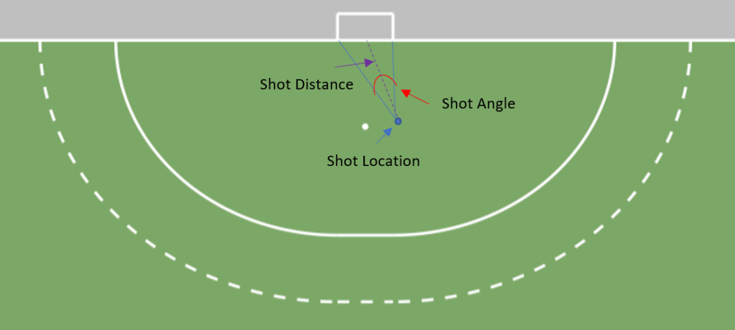
Note. This is a diagram depicting how Shot Distance, Shot Angle, and Shot Location are determined based on the (x,y) coordinates of the shot and center of the goal mouth.
Shot distance (numeric), shot angle (numeric), corner (binary), stroke (binary), deflection (binary), flick (binary), reverse (binary) are all factors considered in the model building process. Of priority for the final model selection is a set of independent variables yielding both a statistically significant fit based on logistic regression, as well as significant model coefficients. The process is run to determine the best fit for both an expected goals (xG) model and expected goals on target (xGOT) model.
Model 1 – xG
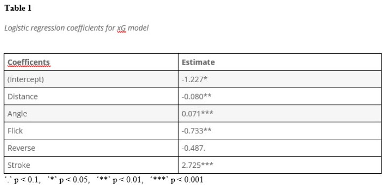
The first of two models created is for the standard expected goals (xG). The binary target variable (Y) is whether or not a goal was scored on a shot (1 – goal, 0 – no goal). After examination of all key independent variables included, the final model is comprised of the following: X1 = Distance (yards), X2 = Angle (degrees), X3 = Flick (1 – yes, 0 – no), X4 = Reverse (1 – yes, 0 – no), X5 = Stroke (1- yes, 0 – no). Using R, the following five predictor logistic model is carried out to determine significance.
The results from R are summarized in Table 1 below:
Overall, the model exhibits a high level of significance. As to the interpretation of the coefficients (given the null deviance of 906.55 on 1011 df and residual deviance of 777.68 on 1006 df), the distance coefficient of -0.080 implies that for every additional yard away from the goal that the shot is, the odds of a goal decrease by about 8%. The shot angle coefficient of 0.071 implies that the odds of a goal increase about 7% for every additional degree in shot angle. The Flick coefficient of -0.733 implies that the odds of a goal decrease about 52% when considering a flick shot vs. a non-flick shot. The Reverse coefficient of -0.487 implies that the odds of a goal decrease about 39% when considering a reverse shot vs. a non-reverse shot. Lastly, the stroke coefficient of 2.724 implies that the odds of a goal increase 1400% when considering a shot off a stroke vs. not a shot off stroke.
Model 2 – xGOT
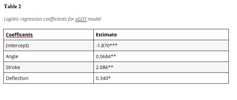
The second of two models created involves the post-shot expected goals, otherwise known as expected goals on target (xGOT). With this model, off target shots automatically receive an xGOT value of 0. Again, the binary target variable (Y) is whether or not a goal was scored on a shot (1 – goal, 0 – no goal). The shots used for model fitting are conditioned for being on target. The following three predictor variables are included in the final model: X1 = Angle (degrees), X2 = Stroke (1 – yes, 0 – no), X3 = Deflection (1 – yes, 0 – no). Using R, the following three predictor logistic model is carried out to determine significance for the xGOT model:
The results from R are summarized in Table 2 below:
Overall, the model exhibits a high level of significance. As to the interpretation of the coefficients (given the null deviance of 711.60 on 602 df and residual deviance of 636.07 on 599 df), the Shot Angle coefficient of 0.068 implies that for every additional meter away from the goal that the shot is, the odds of a goal increase by about 7% given that the shot is on target. The Stroke coefficient of 2.08 implies that the odds of a goal increase about 700% when considering a stroke shot vs. a non-stroke shot given the shot is on target. The Deflection coefficient of 0.785 implies that the odds of a goal increase about 119% when considering a deflected shot vs. a non-deflected shot given the shot is on target.
RESULTS
The model building process exhibits the significance of the logistic regression models in the development of the xG and XGOT metric. In application to the full data sets, both metrics perform well in measuring shot quality, as evidence by an increased association with success.
xG and XGOT average levels on goals vs. non-goals
One way to examine the significance of the xG and xGOT metrics by evaluating at average level splits in goal vs. non-goal occasions. Table 3 shows the xG and XGOT average levels for shots resulting in goals vs. non-goals:
This summary indicates from the sample that shots that were goals had an average xG value of 0.30 vs. 0.14 for shots that were not goals. For xGOT, the split was similar with goals having an xGOT value on average of 0.29 and non-goals have only 0.14 on average. Both of these splits are statistically significant (p-values virtually zero on 2 sample t-test) and are evidence to suggest that higher xG and xGOT valued-shots having higher associations with goal scoring outcomes.
xG and xGOT correlation to goals scored
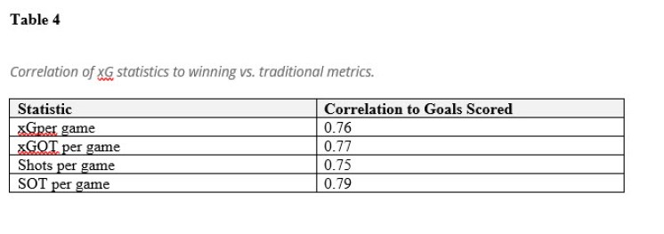
There are 78 observations of team aggregates of goal scored based on a sample of 39 Division I Field Hockey games. Of particular interest is how the xG and xGOT metrics correlate to actual goals scored in a game. Furthermore, the metric correlations to goals scored are also compared to that of traditional counterpart measures such as total shots and total shots on target (SOT). Table 4 below summarizes the correlations of xG per game, xGOT per game, shots per game, and SOT per game to goals scored:
While the results do show evidence of a strong association between xG and xGOT to actual goals scored, there is not much difference between the pairwise relationships of goals scored to either shots per game or SOT per game. Therefore, while xG and xGOT models can do well in measuring shot quality and providing a value that resembles actual goals, there is not clear evidence that they are better measures than shots or shots on target as explaining which team would be more dominant in a particular game.
DISCUSSION
This study shows that xG and xGOT can be meaningful metrics to explain performance in terms of chance creation and execution. While other works may indicate that both xG and xGOT are more highly correlated with goals scored or winning, there is no evidence of a significant difference in correlation to goals scored in this study. The value of xG and xGOT as performance metrics in field hockey can be thought of as more complementary to Shots and SOT. By having all four metrics to describe and explain chance creation and execution, one can have a more complete understanding of quantity and quality in a particular match and throughout a season. Figure 2 below is a sample visual of how the four metrics could be combined as a post-match reporting technique for the Villanova vs. Providence game that took place September 17th, 2021.
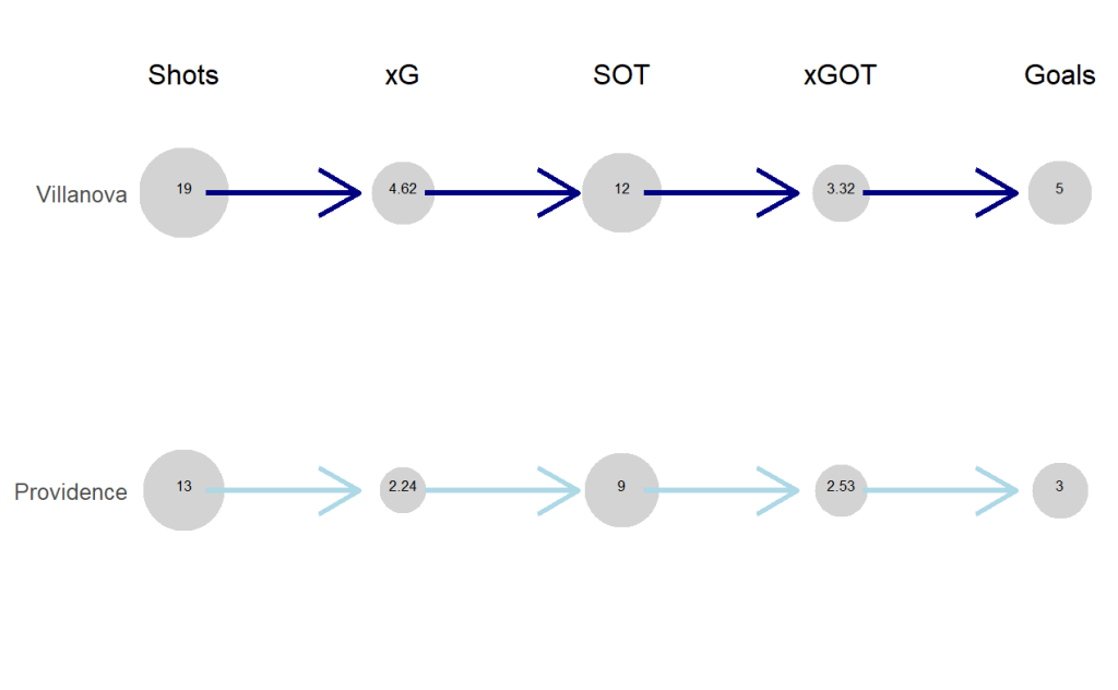
Note. The is a diagram that can be used for post-match analysis where the size of the circles that contain the values for each performance metric are in direction relation to the magnitude of the metrics. The data is from the Villanova vs. Providence game on September 17, 2021.
This diagram provides an intuitive sequence for the reader. From Villanova’s perspective, the team created 19 shots that had an xG value of 4.62. In other words, based on the 19 shots created, Villanova could have expected to score 4-5 goals. In terms of shot execution, 12 of the 19 shots were on target. The 12 shots on target yield an xGOT value of 3.32. In other words, Villanova could expect 3-4 goals based on the shots on target created and executed. Lastly, the diagram flow ends with the 5 actual goals scored by Villanova. This signifies that Villanova was slightly fortunate to end up with 5 goals based on the chances created and how they were executed. Villanova either benefited from good chance execution on target or arguably poor goalkeeping from Providence.
Post-match visuals that feature the field of play are also effective in engaging the reader by adding more context and spatial implications. Figure 3 depicts and open play shot chart for Villanova while Figure 4 is specific to corner shots for Villanova.
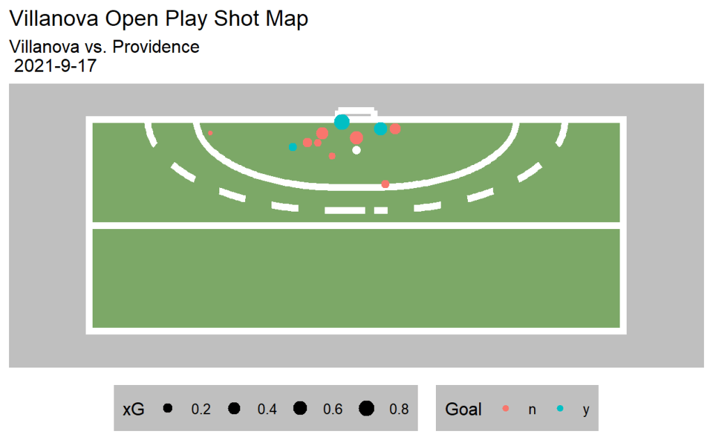
Note. This is an open play shot map where the red points represent non-goal shots and the blue points are goal. The size of the point is in relation to the xG values. The data is from the Villanova vs. Providence game on September 17, 2021.
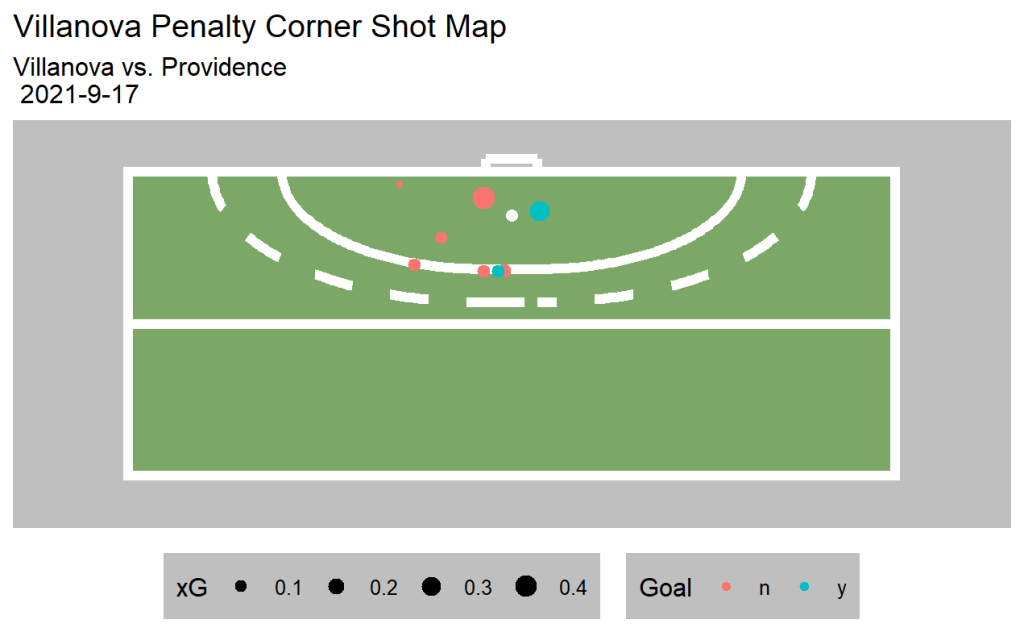
Note. This is a shot map during corner occasions where the red points represent non-goal shots, and the blue points are goal. The size of the point is in relation to the xG values. The data is from the Villanova vs. Providence game on September 17, 2021.
It is apparent that xG plays a role in this visualization as it is represented by the size of the points that represent each shot. Furthermore, shots that were goals are highlighted by being colored differently from shots that are not goals.
One key limitation of this study is that the model coefficients are tailored to Division I field hockey and can have significantly different implications when fitted for other competition levels in global field hockey. It is for this reason that the emphasis of this study is not necessarily on the signs and magnitude of the coefficients that comprise the models. For example, reverse shots have a negative coefficient in the xG model for this study. This result implies that taking a reverse shot results in a lower probability of scoring compared to non-reverse shots. This case may be reflective of the particular skill level of teams in the Division I field hockey sample, which could possibly vary in higher skilled competitions like the Olympics or World Cup where shooters are likely much more effective in executing reverse shots. In addition, there could be a different set of independent variables that turn out to be significant in either the xG or xGOT models when using different shot data. While these caveats are acknowledged, this does not take away from the viability of the application and development of an xG model for Field Hockey.
CONCLUSIONS
The expected goals framework has its place in field hockey as is exhibited by the significant results obtained in this isolated study. Field hockey organizations should acquire the resources necessary to collect detailed shot data so that they have the key variables and analytic prowess to undergo the xG modeling process. While the analysis focuses on the benefits to team evaluation and post-match analysis, the xG and xG metrics can also be extended to player evaluation. The results and implications are not just on the attacking side of the ball, but also, can be used for measuring team defending and individual goalkeeping. Furthermore, coaches and analysts could elect to use xG metrics and implications as an educational tool for players to make better decisions with regards to shot selection.
APPLICATIONS IN SPORT
The expected goals methodology described in this study can be used at high levels of the sport of field hockey (college or professional), given appropriate data collection. Coaches and other key management personnel can use the derived metrics for team evaluation and post-match analysis.
REFERENCES
- Amjad, I., Hussain, I., & Asadullah, M. (2013). Comparison between long corners and short corners in field hockey. Rawal Medical Journal, 38(4), 428-431
- Altman, D. (2014, December 24). Expected goals from situations [Blog]. North Yard Analytics. http://www.northyardanalytics.com/blog/2014/12/24/expected-goals-from-situations/
- Altman, D. (2015). Beyond shots: A new approach to quantifying scoring opportunities. Opta Pro Forum. https://northyardanalytics.com/Dan-Altman-NYA-OptaPro-Forum-2015.pdf
- Ariff M, Norasrudin S, & Rahmat A, (2014) Passing sequences towards field goals and penalty corners in men’s field hockey. Journal of Human Sport Exercise, 10, 638–647.
- Caley, M. (2015, April 10). Let’s talk about expected goals. SB Nation | Cartilage Free Captain. https://cartilagefreecaptain.sbnation.com/2015/4/10/8381071/football-statistics-expected-goals michael-caley-deadspin
- Fairchild, A., Pelechrinis, K., & Kokkodis, M. (2018). Spatial analysis of shots in MLS: A model for expected goals and fractal dimensionality. Journal of Sports Analytics, 4(3), 165–174. https://doi.org/10.3233/JSA-170207
- Laird, P. & Sutherlands, P. (2003). Penalty Corners in field hockey: a guide to success. International Journal of Performance Analysis in Sport, 3, 19-26
- Lord, F., Pyne, D., & Welvart, M. (2022). Field hockey from the performance analyst’s perspective: A systematic review. International Journal of Sports Science and Coaching, 17(1), 220- 232
- Macdonald, B. (2012). An Expected Goals Model for Evaluating NHL Teams and Players. Proceedings for MIT Sloan Sports Analytics Conference 2012. http://hockeyanalytics.com/Research_files/NHL-Expected-Goals-Brian-Macdonald.pdf
- Myers, B., Burnes, M., Couglin, B., & Bolte, E. (2021) On the Development and Application of an Expected Goals Model for Lacrosse. The Sport Journal. September 17th, 2021.
- Piñero, M., Molinuevo, JS., Román, IR. Differences between international men’s and women’s teams in strategic action of the penalty corner in field hockey. International Journal of Performance Analysis in Sport, 7, 67-83
- Rathke, A. (2017). An examination of expected goals and shot efficiency in soccer. Journal of Human Sport and Exercise, 12(Proc2), 16.https://doi.org/10.14198/jhse.2017.12.Proc2.05
- Sunderland, C., Bussell, C., Atkinson, G., Alltree, R., & Kates, M. (2006). Patterns of play and goals scored in international standard women’s field-hockey. International Journal of Performance Analysis in Sport, 6(1), 13-29.

