Abstract

While considerable academic attention has been given to the college selection process of student athletes, it has typically relied strictly on survey responses to determine the relative importance of numerous factors. This research applied means-end theory to the problem of understanding college selection among female student athletes at an NCAA Division II university. Through interviews with participants (N=25), the researchers were able to utilize the laddering technique (Reynolds & Gutman, 1988) to identify not only attributes of the university that were salient to the participants as they made their college selection, but also to probe deeper to determine the underlying values that made the factors important. The values cited by participants were security, achievement, belonging, and fun and enjoyment. This study highlights the function of means-end analysis to investigate college selection among student athletes going beyond the superficial identification of important factors. Via means-end interviews, researchers can determine why varied factors are important to individuals.

Review of Literature

College selection is often a difficult process for students in general and is even more complicated for student athletes, particularly those who are recruited by numerous schools (Klenosky, Templin, & Troutman, 2001). To date, considerable academic attention has been paid to assessing the relative importance of factors student athletes consider during their college selection process. The traditionally used method has been to present student athletes with a survey through which various factors were rated. The factors receiving the highest mean scores were then considered to be the most important to the prospects at the time that they made their final college selection. Factors that were commonly cited as important in the college-selection literature in regard to student athletes were concisely detailed in Kankey and Quarterman (2007), and included: (a) opportunity to play (Forseth, 1987; Johnson, 1972; Konnert & Geise, 1987; Slabik, 1995); (b) academic factors (Bukowski, 1995; Cook, 1994; Forseth, 1987, Mathes & Gurney, 1985; Reynaud, 1998; Slabik, 1995); (c) amount of scholarship (Doyle & Gaeth, 1990; Ulferts, 1992); and (d) head coach (Cook, 1994; Mathes & Gurney, 1985; Slabik, 1995).

Recent studies in this area utilized the traditional method for college selection studies. In both studies, Finley (2005), and Kankey and Quarterman (2007), original surveys were constructed and tested for validity and reliability. Surveys were then distributed in packets to coaches with an accompanying cover letter, instructions for administering the survey, and an addressed and stamped return packet. Both studies utilized five-point scales to elicit scores intended to reflect relative importance of numerous factors. Kankey and Quarterman (2007) elected to use a scale ranging from 5 (extremely important) to 1 (unimportant), while the scale used by Finley (2005) was a traditional Likert scale, ranging from 5 (very important) to 1 (very unimportant), with a neutral category.

Karney and Quarterman (2007) surveyed members of NCAA Division I softball teams in Ohio. Participants (N=196) represented 10 of the 11 programs in the state. The descriptive analysis demonstrated that this population considered availability of major or academic program, head coach, career opportunities after graduation, and social atmosphere of the team to be the most important college choice factors, with the mean score for each being above 4 (very important).

Finley (2005) sought to determine the most salient aspects of college selection among NCAA Division III cross country runners (N=427) from around the country. Results indicated that academic reputation, major or degree program, atmosphere of the campus, and the success of the cross country program were the most important. Finley (2005) also determined that the importance of team-related factors was related to the gender and ability of the athletes. Finley split the sample by gender and then subdivided each gender-group into higher and lower ability groups based on the best cross country time each participant had recorded in high school. Several factors proved to be more important to higher ability males than the other groups: The team’s performance in the prior season, the team’s performance over the last several seasons, the performance of individuals on the team last year, and the number of award-winning athletes from the program were all more important to higher-ability males than to lower-ability males or female cross country runners in both the higher and lower ability groups.

While the aforementioned research was important and contributed to the understanding of the college selection of student athletes, it did not address the question of why these factors are important. Klenosky, Templin, and Troutman (2001) introduced a new strategy for assessing college selection criteria with an eye for understanding the underlying values of the student athletes at the time they selected a college. Specifically, the researchers sought to address the “why” question through interviews with 27 NCAA Division I football players at a single university. Their application of means-end theory (Gutman, 1982) demonstrated that college-selection research can move beyond the survey format to answer the more robust question of why particular factors are important to specific participants. The football players described such factors as facilities, the coach, schedule, and academics as important. Players linked these factors to such consequences as getting a good job, personal improvement as a player, playing on television, and feeling comfortable. In turn, these consequences supported the football players’ values of feeling secure, a sense of achievement, a sense of belonging, and having a fun and enjoyable experience. While Klenosky, Templin, and Troutman (2001) successfully introduced Gutman’s means-end theory to the study of college selection by student athletes, they acknowledged that further studies should explore other levels of competition, and female student athletes. This research sought to make that contribution to the college selection literature.

Means-End Theory

Developed by Gutman (1982), means-end theory allows researchers to explore consumer choice beyond the superficial level to understand the emotional underpinnings that drive consumers’ decisions. Through interviews, researchers guide participants through levels of abstraction, moving from the superficial factors that guide their choice, to the consequences that they perceive will arise (consumers seek to maximize positive outcomes) from their choice, and finally to the personal values they are attempting to reinforce. From each attribute of a program or school that an interviewee describes as important, a means-end chain is created to explore the interconnections between the attribute, the anticipated consequences that arise from the attribute, and finally to the personal value being reinforced. The defining aspect of an interview utilizing this theory is to present the participant with the simple question, “Why is that important to you?” After they name a factor or attribute that was important in their college selection, the researcher simply seeks to determine why that factor was important. This generally leads to a connection to a consequence. Asking why the consequence was important leads into further abstraction, to a statement of a value.

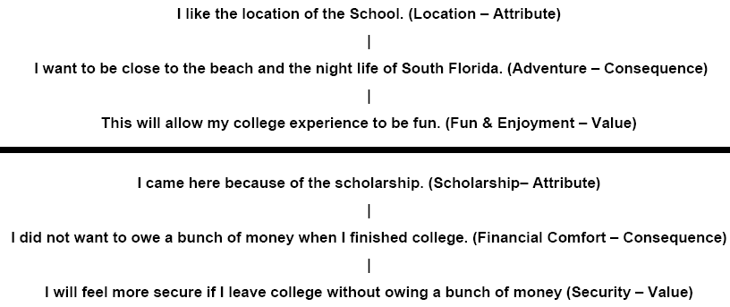
According to the theory, individuals base decisions on factors that are likely to lead to desired consequences (Gutman, 1982). The privileging of one consequence over another reflects the value set of the person empowered with the choice, and they will make selections that reinforce what they have deemed valuable (Klenosky, Templin, & Troutman, 2001). While two athletes might cite the location of a school as an important factor on a traditionally used survey format, it would be unclear whether they value location because of proximity to family, the effect of weather on their sport performance, preference for a rural or suburban lifestyle, or for myriad other reasons. Through the application of means-end theory, researchers can make this determination. As applied to college selection, for example, an athlete might rate facilities as an important factor (attribute) in her college selection. Further questioning (via the “why is that important” question) can elicit the response that facilities were import because she believed it would help her play better (consequence). Finally, she might describe that playing better would reinforce her desire for personal achievement (value). See Table 1 for an example of interview responses and the corresponding coding.

Table 1

Example of two interview ladders and the corresponding coding for each

The present study sought to apply means-end theory to determine the attributes, consequences, and values that underpinned college selection for female student athletes at an NCAA Division II institution.

Semi-structured interviews were conducted with two researchers and individual student athletes. The participants were asked to recall the colleges that they seriously considered as they made their final college selection. Participants were then asked to list factors (attributes) that they relied on as they selected their college over their other finalists. The researchers then utilized the laddering technique as described by Reynolds and Gutman (1988) and later applied to student athletes and college selection by Klensoky, Templin, and Troutman (2001) to create means-end chains, in which each attribute was explored via the question, “Why is that important to you?” This would elicit a response suggesting how this attribute would benefit the participant (consequence). Then the “Why is that important to you?” question would be used to move the participant into deeper reflection, moving from the consequence to a personal value. Participants would create from two to four chains and interviews generally lasted ten to fifteen minutes.

To elicit the most thoughtful and honest answers possible, the researchers utilized the interview methods suggested by Reynolds & Gutman (1988). These included conducting interviews in a non threatening environment (a library area was used, which represented a more neutral site for participants than would a professor’s office or a classroom), making an effort to position the participant as the only expert regarding their college selection, with emphasis being placed on reassuring them that there was no right or wrong answer, and showing interest in responses while refraining from giving cues suggesting judgment. Following each interview, the researchers used interview notes to create means-end chains, which connected each attribute cited by the participants with the corresponding consequences and values stemming from it. Discrepancies were resolved jointly, relying as strictly as possible on key words and phrases used by the participants and recorded in the interview notes.

Participants

The participants in this study were 25 female student athletes at an NCAA Division II university in Florida during the 2005-2006 academic year. Participants represented a variety of sports, including basketball, soccer, softball, golf, tennis, rowing, and cross country.

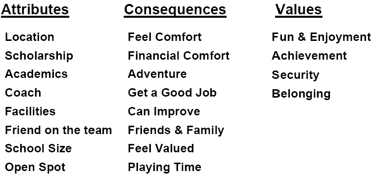
In total, 77 means-end chains were created, an average of 3.08 per participant. Coding of the means-end chains revealed eight attributes cited as important to the selection of the student athletes’ current college. These attributes led to eight potential consequences, which, in turn, led to four values.

Table 2

Summary of all attributes, consequences, and values identified throughout the interview process

Using the coded data, an implication matrix was constructed (Table 3) as a summary of the connections between attributes, consequences, and values. In addition to showing the number of participants that mentioned a concept (under N), the matrix also lists the number of total times the concept was mentioned. Each cell reflects the number of times the concept was mentioned. For example, location linked to the consequence of feel comfort (C1), three times and connected to the consequence of adventure (C3) twelve times. Location also connected to the value fun and enjoyment (V1) fifteen times. The implication matrix was then used to construct a Hierarchical Value Map (HVM).

table 3

Implication Matrix for female student athletes’ college selection

As information from the implication matrix was transferred into the HVM, the researchers selected a cutoff level of two. A cutoff level establishes how frequently a connection had to be made to be depicted in the HVM. Thus, only connections made two or more times are illustrated with a line. Eliminating connections made only one time reducing clutter in the HVM. To assist the reader in interpreting the HVM, an illustrative example is presented (Figure 1). The complete HVM follows (Figure 2). Consistent with the literature (Klenosky, Templin, & Troutman, 2001), values are presented at the top of the map to represent their abstract nature in college selection (they appear within triangles and are spelled with all capital letters). Consequences are represented across the middle (within circles and beginning with a capital letter), and attributes appear at the bottom (within rectangles and all lower case letters) to reflect that they were merely the beginning point in each chain and are the most superficial level of information gathered. Further, the lines between attributes, consequences, and values represent the frequency of the connection between these concepts (more frequent associations depicted with thicker lines). The size of each shape also reflects the number of participants mentioning it, with more frequently mentioned concepts dominating more space. Finally, the first number in each shape reflects the number of participants that mentioned the concept, while the number in parenthesis is the number of times the concept was mentioned in total, reflecting that some concepts would be mentioned multiple times by a single participant.

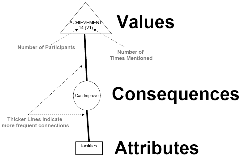
Figure 1. An illustrative example of an HVM section

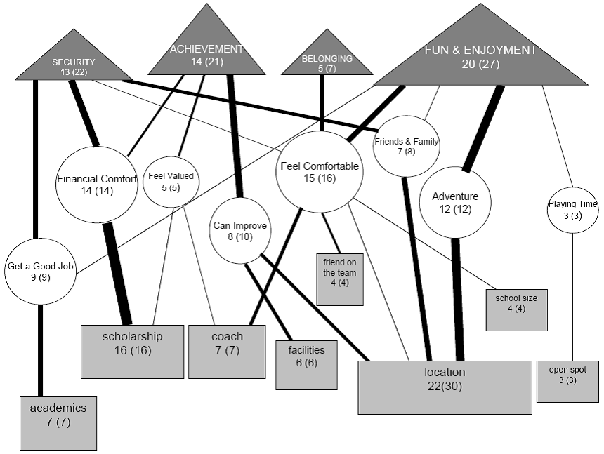
Figure 2. Hierarchical Value Map for female student athletes’ college selection

Analysis of the HVM revealed several noteworthy findings. First, location was a primary attribute for the selection of this university over other universities the athletes considered as they made a final decision. In fact, 39% of all the chains created in this study began with the attribute of location. While it might not be surprising that a university in the state of Florida is selected for its location, this fact underscores the importance of a means-end analysis. While a college selection survey would also reveal that location was important, it would not discover the true reason for the importance of this attribute. The means-end analysis demonstrated that the attribute of location was important for several different reasons. Of the 30 chains beginning with location, 12 went to the consequence of adventure and then continued on to the value of fun and enjoyment. Other participants indicated that location was important because it kept them close to friends and family, which had a strong connection to the value of security. Others expressed that they simply are comfortable here, which largely connected with fun and enjoyment. Finally, some participants (in outdoor sports) noted that the weather in Florida would allow them to improve their sport performance (largely due to an extended season), which supported the value of achievement.

The different values that underpinned the importance of location supported the belief that college selection is a complicated process and that a single attribute of a campus can be important to prospective student athletes for a wide variety of reasons. This fact should be particularly interesting to coaches who spend considerable time and effort in the recruitment process and could misinterpret a prospects’ motivation for selecting a particular university. For example, coaches might feel confident that a student athlete selected a college because of location and may even presume to know that it is related to a consequence, such as improving sport performance, whereas in the mind of the student athlete, lying on the beach might be the true motivator because she is more driven by her value of fun and enjoyment than by the value of achievement.

Second, the attribute of receiving an athletic scholarship was also frequently mentioned. It was important to 16 of the 25 participants (64%). Predominantly it led to the consequence of financial comfort, which, in turn led to the value of security. For a few participants, however, the consequence of financial comfort led to the value of achievement, which reflected their belief that financial comfort was essentially earned through their years of dedication to sport participation. Comments made during the interviews suggested that the participants viewed the scholarship as a literal indication that they had achieved within their sport and that their achievement became measurable and worthwhile through the scholarship offer. Participants reported being offered scholarship packages of widely varying values and thus scholarship became an important attribute in differentiating between schools. The Klenosky, Templin and Troutman (2001) study did not reveal scholarship as an important attribute among the Division I football players because each participant in the sample reported being recruited by over 20 schools and thus scholarship was likely a non-issue in differentiating between schools.

Third, the attributes of the coach and academics were mentioned by surprisingly few participants. These attributes were seldom used by participants to differentiate their school from others at the time they made their final selection. Still, it is interesting to see that these attributes trailed location and scholarship by a wide margin. For the seven participants who mentioned academics, all of them linked it to the consequence of getting a good job, as opposed to more altruistic notions such as gaining knowledge or growing as a person.

Fourth, the consequence of feeling comfort was frequently mentioned and stemmed from a variety of attributes. School size, location, a friend on the team, and the coach were all attributes that seemed to assure the participants that this school would be a good fit for them and provide a place in which they would feel comfort. This information is valuable for coaches who actively recruit prospects. It is possible that a key to securing recruits is in convincing them that the attributes of the college, team, and campus will help the prospect feel comfort.

Fifth, the value of fun and enjoyment underpinned the college selection for many participants (it was mentioned by 20 of the 25 participants (80%), and several participants had multiple chains end with this value). However, the source of fun and enjoyment was extremely varied. At the time the college selection was made, participants believed that playing time, adventure (from location), proximity to friends and family, a comfortable atmosphere, and opportunity to get a good job all led to the possibility of fulfilling the value of fun and enjoyment.

This study contributes to the college selection literature and furthered the work of Klenosky, Templin, and Troutman (2001) to utilize means-end theory to determine the values that student athletes rely on in this process. However, there were limits to the study. Most notably, it only represented student athletes from one university and results do not generalize to female student athletes overall. Different results could occur among student athletes at other schools based on such traits as school size, region of the country, and NCAA division.

College selection is a complicated and difficult process for student athletes, which is often made even more confusing by the recruitment process. While traditionally researchers have sought to understand college selection by drawing from sizable data sets gathered via surveys, that method fails to explore fully the complexity of any given attribute (such as location). By applying means-end theory researchers can probe further and determine the values on which prospects are basing their selection. Further, a general understanding of means-end theory could be important for coaches to improve the process of attracting prospects in an increasingly competitive college sports climate. It also can assist coaches in understanding what is important to the student athletes once they matriculate to campus.

For the participants in this study, security, achievement, belonging, and fun and enjoyment were the guiding values for college selection. Future research should extend the use of means-end analysis to student athletes in other contexts, for example by sport, NCAA division, and region of the country.

Bukowski, B. J. (1995). Influences on student college choice for minority and non minority athletes at a Division III institution (Doctoral dissertation, University of Wisconsin, Madison, WI). Dissertation Abstracts International, 56(7), 126.

Cook, T. (1994). Factors female freshmen student-athletes use in deciding between a NJCAA college and a NAIA college. Unpublished master’s thesis, University of Kansas, Lawrence, KS.

Doyle, C. A. & Gaeth, G. J. (1990). Assessing the institutional choice process of student athletes. Research Quarterly for Exercise and Sport, 61(1), 85-92.

Finley, P. S. (2005). An analysis of team Web site content and college choice factors of NCAA Division III cross country runners (Doctoral dissertation, University of Northern Colorado, Greeley, CO). Dissertation Abstracts International, 66(04), 1291.

Forseth, E. (1987). Factors influencing student-athletes’ college choice at evangelical, church-supported NAIA institutions in Ohio (Doctoral dissertation, The Ohio State Univesity, Columbus, OH). Dissertation Abstracts International, 48(01), 172.

Gutman, J. (1982). A means-end chain model based on consumer categorization processes. Journal of Marketing, 46(2), 60-72.

Johnson, E. A. (1972). Football players’ selection of a university. Unpublished master’s thesis, University of Utah, Salt Lake City, UT.

Kankey, K., & Quarterman J. (2007). Factors influencing the university choice of NCAA Division I softball players. The SMART Journal, 3(2), 35-49.

Klenosky, D. B., Templin, T. J. & Troutman, J. A. (2001). Recruiting student athletes: A means-end investigation of school-choice decision making. Journal of Sport Management, 15, 95-106.

Konnert, W., & Geise, R. (1987). College choice factors of male athletics at private NCAA Division III institutions. College and University, 63(1), 33-44.

Mathes, S., & Gurney, G. (1985). Factors in student-athletes’ choice of colleges. Journal of College Student Personnel, 26(4), 327-333.

Reynaud, C. (1998). Factors influencing prospective female volleyball student-athletes’ selection of an NCAA Division I university: Towards a more informed recruitment process (Doctoral dissertation, Florida State University, Tallahassee, FL). Dissertation Abstracts International, 59(02), 445.

Reynolds, T. J., & Gutman, J. (1988). Laddering theory, method, analysis and interpretation. Journal of Advertising Research, 28(1), 11-31.

Slabik, S. L. (1995). Influences on college choice of student-athletes at National Collegiate Athletic Association Division III institutions. Unpublished doctoral dissertation, Temple University, Philadelphia, PA.

Ulferts, L. (1992). Factors influencing recruitment of collegiate basketball players in institutions of higher education in the upper Midwest (Doctoral dissertation, University of North Dakota, Grand Forks, ND). Dissertation Abstracts International, 54(03), 770.

Authors Note:
Correspondence for this article should go to Peter Finley, H. Wayne Huizenga School of Business and Entrepreneurship, 3301 College Avenue, Fort Lauderdale-Davie, Florida 33314, (954) 262-8115, pfinley@huizenga.nova.edu.

References

Baron, J. (200). Thinking and Deciding, 3rd edition, Cambridge, UK: Cambridge University Press.
Elster, J. Ed. (1986). Rational Choice. Oxford, UK: Basil Blackwell.
Fishbein, M. and Ajzen, I. (1975). Belief, Attitude, Intention, and Behavior: An Introduction to Theory and Research. Reading, MA: Addison-Wesley.
Goodman, G.F. (2006). Five common email marketing mistakes. http:// www.Entrepreneur.com>
Graves, R. (2006), Golf Ranges Drives Profits: Today’s range is a practice center, learning center, clubfitting center, Etc. PGA Magazine, (August 1), 37-57.
Harack, T. (2006), Pushing forward: A proactive recruitment program can help stimulate stagnant membership roles, Golf Business, 12 (August), 26-27.
Hawkins, D., Mothersbaugh, D., and Best, R. (2007). Consumer Behavior: Building Marketing Strategy, 10th ed. Boston, MA: McGraw-Hill: Irwin.
Homans, G. (1961). Social Behaviour: Its Elementary Forms. London: Routledge and Kegan Paul.
Johnson, D., and White, J. (2004). A new integrated model of noncompensatory and compensatory decision strategies, Organizational Behavior and Human Decision Processes, 95, 1-19.
National Golf Foundation (2004), Rounds Played in the United States, 2004 Edition.
National Golf Foundation Press Release (2007), Rounds Played in the United States, 2007, <http://www.ngf.org/cgi/whonews.asp?storyid=191>
Staw, B.M. (1981). The escalation of commitment to a course of action. Academy of Management Review, 6, 577-587.
Von Neuman, J, and Morgenstern, O. (1972). Theory of Games and Economic Behavior, Princeton, NJ: Princeton University Press.
2016-10-19T11:00:39-05:00March 14th, 2008|Sports Facilities, Sports Management, Sports Studies and Sports Psychology|Comments Off on Retaining Current Vs. Attracting New Golfers: Practices among the Class A Carolinas Professional Golf Association Membership
Show Me the Money! A Cross-Sport Comparative Study of Compensation for Independent Contractor Professional Athletes
Abstract:
Numerous pay equity studies have been conducted. Many have examined the compensation of professional athletes. However, few studies have compared athlete compensation across sports, which is the objective of this research. Focusing on independent contractor athletes, several analyses were performed to determine how one type of athlete’s (e.g., horse jockeys) earnings from competition (excluding sponsorships, appearance fees, etc.) compare to other types of contracted athletes, such as race car drivers, golfers, bull riders, tennis players, etc. Overall, this exploratory study sheds insight into how the different groups of athletes are paid, and, more importantly, provides a framework for future research that examines the compensation inputs (versus outputs) of each of these groups.
Introduction:
Salaries for professional athletes continue to escalate each year. From Alex Rodriguez’s record $252 million contract to David Beckham’s $50 million per year enticement to join the LA Galaxy soccer team, most sports fans believe that professional athletes, in general, are overpaid and not worth their salaries. Yet for the professional athlete, maximizing compensation is critical, given the short careers and health risks associated with professional sports. Thus, athletes and their agents often look to see what others within their sport are paid in an effort to negotiate for more money. Few, if any, have compared athlete compensation across sports. While a cross-sport comparison might not be necessary in team professional sports (e.g., MLB, NHL, NFL, NBA) given the strength of their collective bargaining agreements, independent contractor professional athletes (e.g., jockeys, bull riders, golfers, race car drivers) need this type of analysis. The purpose of this research is to compare independent contractor professional athlete salaries across sport using four perspectives: total payout to athletes per sport, percentage of winnings per sport, top individual earner by sport and mean earnings for the top 50 athletes in each sport. These perspectives will allow independent contractor professional athletes to better analyze the “fairness” or equity of compensation.
Background:
Ever since jockey Gary Birzer was paralyzed while racing in 2004, the jockeys’ guild and track owners have had an acrimonius relationship, to say the least. While much of the ongoing battle has centered on who should pay for the jockeys’ long-term disability coverage, the dispute has recently turned to jockey compensation. The jockeys believe they are underpaid, given the amount of overall purse money involved in the sport and the inherent health risks of racing horses. In contrast, the race tracks believe that the horse owners and trainers deserve the bulk of winnings, given their financial risk and knowledge. With the sides at a stalemate, Corey Johnsen, President of Lone Star Park at Grand Prairie and current President of the Thoroughbred Racing Associations (the trade organization for the tracks) commissioned this study. By collecting extensive data across a number of sports, Johnsen sought to provide a starting point for discussions between the tracks and the jockeys’ guild in an effort to resolve the dispute.
References:

Carrell, M. and J. Dittrich (1978). Equity theory: The recent literature, methodological considerations, and new directions, The Academy of Management Review, Vol. 3, 202.
Idson, T. and L. Kahane (2004). Teammate effects on pay, Applied Economics Letters, Vol. 11 (12), 731.
Nero, P. (2001). Relative salary efficiency of PGA tour golfers, American Economist, Vol.45 (2), 51.
Porter, P. and G. Scully (1996). The distribution of earnings and the rules of the game, Southern Economic Journal, Vol. 63 (1), 149.
Scully, G. (2004). Player salary share and the distribution of player earnings, Managerial and Decision Economics, Vol. 25 (2), 77.
Slottje, D., J. Hirschberg, K. Hayes and G. Scully (1994). A new method for detecting individual and group labor market discrimination, Journal of Econometrics, Vol. 61 (1), 43.
St-Onge, S. (2000). Variables influencing the perceived relationship between performance and pay in a merit pay environment, Journal of Business and Psychology, Vol. 14 (3), 459.
Sweeney, P. and D. McFarlin (2005). Wage comparisons with similar and dissimilar others, Journal of Occupational and Organizational Psychology, Vol. 78, 113.
Younts, C.W. and C. Mueller (2001). Justice processes: Specifying the mediating role of perceptions of distributive justice, American Sociological Review, Vol. 66 (1), 125.
2016-10-20T10:28:15-05:00March 14th, 2008|Contemporary Sports Issues, Sports Management, Sports Studies and Sports Psychology|Comments Off on Show Me the Money! A Cross-Sport Comparative Study of Compensation for Independent Contractor Professional Athletes
Cross-Country Skiing USSA Points as a Predictor of Future Performance among Junior Skiers
Junior cross-country skiers’ performances prior to participation in the 2006 Junior Olympics were compared to their results in the 2006 Junior Olympics using USSA points as a measure of performance.  Junior class and division (team) were also included as independent variables.  Prior performance as determined by USSA points is a poor indicator of performance in the Junior Olympics.
Cross-country skiing times from different races, even those of the same length, are not comparable because the terrain is different for each race.  Furthermore, snow conditions may vary, even from hour to hour, on the same course.  Merely comparing times of skiers over similar distances is not an accurate comparative assessment of skiers’ abilities.  The United States Ski and Snowboard Association (USSA) points list was developed to allow comparison between skiers who may have entered several different races.  USSA points are awarded to registered cross-country skiers for participation in sanctioned ski races.  A lower value in USSA points indicates that a skier is a better, more competitive skier.  USSA points and similar International Ski Federation (FIS) points are used to help select the U.S. national teams, to seed racers in both mass and interval start races, and to monitor the progress of athletes in physiological studies (Bodensteiner & Metzger 2006; Staib, Im, Caldwell, & Rundell 2000).
The USSA formula that allocates points to skiers is based on race performance. It includes a number of variables that capture the relative ability of skiers in the race.  Who enters the race and how they place are used in determining the penalty.  Each race’s penalty is based upon the current USSA points of top finishers in the race.  The type of start or race and a minimum penalty also are used in the calculation of USSA and FIS points assigned to a skier’s race (Bodensteiner & Metzger 2006, International Ski Federation, 2006).  Despite the common and, at times, mandatory use of the system, the USSA point system has been criticized by racers and coaches over the years for failure to accurately capture a skier’s ability (Anonymous, 2006; Smith, 2002; Trecker 2005).
Methods:
Given the importance and criticism of USSA points, this study develops a systematic comparison of prior USSA points results of skiers to their USSA points earned in a common competition.  One would hypothesize that a skier’s points prior to a competition would predict a skier’s points earned within the competition.   Points earned by Junior skiers (ages 14 to 19) in the 2005-2006 season are compared to USSA points in the 2006 Junior Olympics.  The use of linear regression allows one to determine if a linear relationship exists between prior performance and performance in the Junior Olympics and whether other, easily obtained variables can improve the ability to predict performance at the Junior Olympics.  (Hill, Griffiths, & Judge, 1997; Johnston, 1984)
Before the Junior Olympics, skiers earned USSA points in different races throughout the northern part of the United States.  Skiers within any of the ten USSA districts competed against each other, but there was limited competition among skiers from different districts.  The top 400 skiers then competed in the Junior Olympics in March, 2006 in Houghton, Michigan.  The end of season Junior Olympics allows skiers to be directly compared on the same course and with the same snow conditions, so USSA points assigned in these races can be used in this study free of the bias of course and snow conditions.
A general linear model (equation 1) with USSA points earned in the Junior Olympics as the dependent variable and USSA points prior to the Junior Olympics, junior class (J2, J1, or OJ) division (team) were used as independent variables.  The parameters c and ak (where k = 1, 2, and 3) were estimated.  Estimated parameters in bold are matrices of parameters associated with a matrix of dummy variables.  Equation 1 is the most comprehensive linear model used.
yi = c + a1*Pi + a2* JCLASSi + a3*DIVi + ei          equation 1
Where
yi = USSA points in the 2006 Junior Olympics for the ith skier,
c = an estimated constant,
Pi = USSA points prior to the Junior Olympics for the ith skier,
a1 = the estimated parameter associated with Pi,
JCLASSi = a matrix of junior classes with dummy variables for OJ, J1, and J2 where the value is 1 in the ith skier’s junior class and zero for other classes,
a2 = a matrix of estimated parameters associated with JCLASSi,
DIVi  = a matrix of regional divisions with dummy variables for Alaska, Great Lakes, Midwest, Intermountain, Rocky Mountain, Mid-Atlantic, New England, Far West, High Plains, and Pacific Northwest where the value is 1 in the ith skier’s division and zero for other divisions,
a3 = a matrix of estimated parameters associated with DIVi, and
ei = the residual value for the ith skier.
The model was run using USSA points from all three individual races at the Junior Olympics (yi): freestyle, classic, and sprint.  USSA points prior to the Junior Olympics included (Pi) for distance, sprints, and overall points were used in separate regressions.  Thus, there are several versions of equation 1 that use different techniques (classic and freestyle) and USSA disciplines (sprint, distance, and overall).
While equation 1 represents the most extensive model tested, other models using a subset of the independent variables were also tested to determine the stability of the model.  When sets of independent dummy variables would have resulted in a full rank matrix, one of the variables was not included in the regression.   Technical definitions associated with cross-country skiing terms can be found in the USSA’s Nordic Competition Guide (Bodensteiner & Metzger, 2006). Analyses were run using the GLM procedure in SAS 9.1 for Windows.
Data:
Pre-Junior Olympics distance, sprint, and overall USSA points; names; USSA numbers (to confirm this data with results from the Junior Olympics); junior class (J2, J1, or OJ); and year of birth information were obtained from the national list of USSA points, which had been updated just prior to the Junior Olympics.  Data were downloaded on March 27, 2006.  Junior Olympic classic, freestyle, and sprint USSA points; skier’s division (team); name; and USSA number were obtained from itiming.com via the web in the week following the 2006 Junior Olympics.  In all cases, as complete a data set as possible was used in the regression.  However, some skiers entered the Junior Olympics without prior USSA points or with only a partial set of information.  The most common missing data were USSA sprint points prior to the Junior Olympics.  Whenever a valid number was available for a skier, that skier was entered in the data set for a particular regression analysis.  In a few cases, skiers did not start or finish a race or were disqualified during the race.  The largest data set included information for 271 skiers.
Results:
USSA Points prior to the Junior Olympics – the simplest models.
The first part of the statistical analysis was to determine if USSA points alone could predict USSA points in the Junior Olympics.  The model used to test this question was:
yi = c + a1*Pi + ei          equation 2
Since skiers have sprint, distance, and overall points prior to the Junior Olympics and compete in sprint, freestyle distance, and classic distance events, there are six logical combinations of dependent and independent variables.  Table 1 shows the results of each regression.
Anonymous.  (2006).  U.S. Olympic Cross Country Team Announced.  Retrieved October 6, 2006 from http://www.fasterskier.com/news2962.html  .
Bodensteiner, L., & Metzger, S.  (2006).  2006 USSA Nordic Competition Guide.  Park City, UT.
Hill, C., Griffiths, W., & Judge, G.  (1997).  Undergraduate Econometrics.   J. Wiley & Sons, New York.
International Ski Federation.  (2006).  Cross Country Rules and Guidelines of the FIS Points 2006/07.  Retrieved October 11, 2006 from http://www.fis-ski.com/data/document/pktrgl0607-neu.pdf
Johnston, J.  (1984).  Econometric Methods (3rd ed.)  McGraw-Hill, New York.
Smith, C.  (2002).  U.S. Olympic Team Selection.  Retreived July 17, 2006 from http://www.xcskiracer.com/rants.shtml
Staib, J.L., Im, J.,Caldwell, Z., & Rundell, K.W.  (2000).  Cross-country ski racing performance predicted by aerobic and anaerobic double poling power.  Journal of Strength and Conditioning 14(3), 282-288.
Trecker, M.  (2005).  Following the Olympic Trials, Who’s Hot, Who’s Not, and the Strange Anomalies of USSA Scoring.  Retrieved July 17, 2006 from http://www.fasterskier.com/opinion2749.html
Appendix – Heteroscedasticity in the Data Set:
This portion of the study on heteroscedasticity is placed in the appendix because most people interested in skiing will not be interested in statistical methods and assumptions.  They want to know if current USSA points predict future skiing results.  However, from an analytical viewpoint, improper use of statistics can lead to incorrect results and correct procedures lead to improved analysis.  One assumption of linear regression is that the variance of the random error term is 2 for all x.  If this is not the case, then the estimate remains linear and unbiased but it is no longer the best linear unbiased estimator and standard errors are often incorrect (Johnston, 1984).  Confidence intervals and results of statistical tests can be misleading.  This appendix covers four topics:  heteroscedasticity in equation 2, correcting for heteroscedasticity using data transformations, heteroscedasticity in the complete data set, and a brief conclusion.
Heteroscedasticity in equation 2
Equation 2 is the intuitive equation to test whether prior performance as measured by USSA points can predict future performance.
yi = c + a1*Pi + ei          equation 2.
Figure 1 shows a much wider variance in the dependent variables as USSA points increase.  White’s test for heteroscedasticity indicates a probability of greater than 99.99% that heteroscedasticity does exist (test statistic= 15.37 with two degrees of freedom).
Correcting for heteroscedasticity using data transformations
Data may be adjusted using transformations to eliminate heteroscedasticity (Hill et al, 1997, Johnston 1984).  In the data set used in this study, the variance in the residuals is larger for the larger values of the independent variable.  Two logical transformations are to take the logarithm of the independent variable and the square root of the independent variable.  Separate regressions were estimated using equation (2) where
(a)  Pi = the square root of the competitors USSA points earned prior to the Junior Olympics and
(b)  Pi = the natural logarithm of the competitors USSA points earned prior to the Junior Olympics.
In both cases, the r2 value improved less than 0.02, and the White’s test indicated that heteroscedasticity remained a problem.
Heteroscedasticity in the complete data set
The complete data set, including division and junior class of the competitor, not only improves the estimation, it is less likely heteroscedasticity exists.  White’s test for heteroscedasticity indicates a probability of approximately 80% that heteroscedasticity does exist (test statistic= 49.46 with 42 degrees of freedom).  Most researchers would not reject the null hypothesis at this level.  This indicates that the additional independent variables have the greatest impact on improving prediction for skiers with the higher (less competitive) prior USSA points.
Conclusion:
The original goal of this study was not only to determine what statistical model would work best for the data, but to determine if USSA points were a good predictor of future performance of athletes.  From a practical standpoint, a complex model used in the prediction would indicate that USSA points alone are a poor predictor and a complex model would be difficult to justify and administer.  The heteroscedasticity and the development of more complicated, but still unstable, models reinforce the results of the main paper.  Prior USSA points are poor predictors of Junior races.
2016-10-20T10:03:26-05:00March 14th, 2008|Sports Coaching, Sports Management|Comments Off on Cross-Country Skiing USSA Points as a Predictor of Future Performance among Junior Skiers