Contemporary Sports Issues – Page 16

The Impact of Hip Rotator Strength Training on Agility in Male High School Soccer Players

Submitted by Jesse Obed Nelson and Mark DeBeliso

ABSTRACT
The strength of the muscles surrounding a joint contributes to the stability of the joint. The stability of a joint provides the foundation for large muscle groups to perform high speed forceful actions. The purpose of this study was to examine if strengthening of the hip rotator muscles could improve measures of agility. Twenty-nine male high school soccer players were recruited to participate in a 9-week matched pair study. The control and the experimental group participated in regular weight training and soccer practice. Additionally, the experimental group performed three sets of the hip rotator exercises using latex chords (medial and lateral rotation) twice per week with both legs. The dependent variables were the T-Test, the Hexagon Test, and the 20-Yard Shuttle Run. All athletes were pre- and post-tested on each of the agility drills. A gain score was then calculated as the difference between pre- and post-test agility scores. An independent t-test was used to determine if there were any differences (p < 0.05) between the experimental and control groups. Statistical analysis showed no significant difference between the two groups for T-test (p=0.12), Hexagon test (p=0.35), and 20-yard shuttle run (p=0.18). The research hypothesis, which stated that adding hip strengthening exercises for the experimental group would produce faster times on the agility tests, was rejected. Possibly the volume of training, which often included three hours of exercise and practice per day, rendered the additional hip strengthening exercises insignificant. Repeating the experiment in the off-season with lower training volume might produce different results. INTRODUCTION
In sport and physical therapy there is not much time spent in training the medial and lateral rotators of the hip, while medial and lateral rotators of the arm (rotator cuff) are regularly exercised (15, 17). The deep inner muscles of the hip are often neglected and overlooked in the development of training programs for all types of sport.

Field sports which might benefit from strengthening of the hip rotators are those which require movements of agility (e.g. soccer, football, lacrosse, rugby, and basketball). Agility requires rapid change of direction. This is where stronger hip rotator muscles may help athletes. An increase in performance might be experienced as a result of stronger hip rotator muscles.

Injury rate reduction might also be a benefit of improving the strength of the hip rotator muscles. Sports that include running, dancing, and hockey are at increased risk of hip injuries (2, 7). Recent investigations suggest that 23% of athletes (e.g. divers, weightlifters, wrestlers, orienteers and ice-hockey players) have experienced a hip injury in the previous year (12). Muscle weakness is an intrinsic risk factor to joint injuries in sport (18). Strengthening of the hip rotator muscles is prehabilitative in nature, much the same as training the internal and external rotator cuff muscles (17). Prehabilitation is a concept where muscle groups are exposed to various exercise protocols with the hope of reducing the occurrence and severity of sport injuries (16, 17). A prehabilitative program for Rugby Union players identified the lower body including the hip as a specific target, however, isolated training of the hip rotator muscles was not included (16).

Internal and external hip rotator muscles include the adductor longus, adductor magnus, biceps femoris, gemellus inferior, gemellus superior, gluteus maximus, gluteus medius, gluteus minimus, gracillis, illiacus, obturator externus, obturator internus, piriformus, psoas, quadratus femoris, sartorius, semimembranosus, semitendinosus, and tensor fascia latae (11). There is a paucity of research examining the role of the hip rotator muscles in sport and prehabilitation. As such, this research effort focused on the impact of incorporating exercises that target the hip rotator muscles on sport-specific agility tests.

The research hypothesis is that, after training, the experimental group will show significant improvements versus the control group on the T-test, Hexagon test, and the 20-yd shuttle run. These tests are indicators of speed and agility (23), and are considered sport performance characteristics of the “best soccer” players (23). Hence, the purpose of adding the hip rotation exercises was to determine if there would be a positive influence on speed and agility. Conversely, the null hypothesis was that the addition of hip rotation exercises to the training program for the experimental group would not yield better performance on the agility drills than the control group.

If the research hypothesis is supported, coaches and athletes might incorporate hip rotator exercises to strength and conditioning regimens leading to improved agility. This research could also provide the foundation for future experiments regarding medial and lateral hip rotator muscles and the relation to sport performance.

METHODS
A convenience sample of male high school soccer players (n=29) was recruited to participate in a 9-week matched pair study. The participants were experienced in weight training, and trained and experienced at the competitive level in the sport of soccer. As such, participant fitness levels were likely above average for those of the same age and gender.

Age, weight, and height were recorded at the pretest. For the experimental group, the average age was 16.3±0.9 years with a range of 15-18 years. The average body mass was 68.1±9.9 kg, with a range of 57-89 kg. The average height was 173.3±8.9 cm, with a range of 165-193 cm. For the control group the average age was 16.6±0.7 years, with a range of 16-18 years. The average body mass was 66.3±8.7 kg, with a range of 54-86 kg. The average height was 173.0±7.7 cm, with a range of 163-188 cm.
Previous exercise history included calisthenics, stretching, running sprints, and weight training (all performed under the supervision of the strength and conditioning coach). The players also played a friendly game (against each other) two times per week before school. The participants were all varsity and junior varsity players, and most had played soccer since elementary school. No players were classified at the beginner level. All had been active and in good physical condition for years before the beginning of the experiment.

Human Subjects Approval was required and obtained. Informed Consent and Parental Consent was also required and obtained before subjects were allowed to participate in the study. Participants were allowed to withdraw at any time. The Informed Consent Document was approved by the University Institutional Review Board.
In order to conduct this study an experimental and control group were formed using a matched pair design (5). All of the participants performed the agility T-test, and then ranked from fastest to slowest. The first two highest scoring participants were matched and randomly assigned to either the experimental or control group. This process was repeated until the experimental (n=14) and control (n=15) groups were completed. This matched pair design assured that the two groups were essentially equal based on initial T-test scores.

Equipment for the strength and conditioning program was that traditionally found in many high school weight rooms. Iron plates were loaded onto weight bars for the squat, the deadlift, and other exercises. All of the athletes in both the experimental and control groups performed the same weight training exercises with the strength and conditioning coach. The training volume was the same for the experimental and control groups with the exception of the additional volume incurred by the experimental group as a result of performing the supplemental internal and external hip rotation exercises.

Weekly workouts during the intervention included 2-3 strength and conditioning sessions per week. The school had a rotating block class schedule, alternating successive weeks with two and three strength and conditioning classes respectively. The soccer team had practice for 1.5 hours every weekday after school unless there was a “friendly game” in the morning. All team members focused on stretching and recovery, but the experimental group still performed the hip rotator exercises.
Strength and conditioning sessions began in the wrestling room with calisthenics including bear crawls, planks, sit-ups, wall sits, push-ups, and some simple jumping drills. The team would then stretch with a focus on the legs. After stretching, half of the team would work with the track coach in the hall, while the other half would work with the strength and conditioning coach to the weight room. The group in the hall performed dynamic stretching and simple footwork drills such as butt-kicks, high knees, grapevines, 10 yard sprints, and skips. The group in the weight room did differing exercises depending on the day, mostly rotating with upper body, lower body, and total body exercises. The total body exercises included dot drills, deadlifts, hang cleans, and power cleans. The dot drills, hang cleans, and power cleans were exercises where members of both groups were encouraged to move as explosively as possible during the execution of the exercises while maintaining proper technique. Upper body exercises included the flat, incline, and decline bench press, push press, military press, dumbbell shoulder press, dumbbell row, dumbbell biceps curl, dumbbell triceps press, and pull-ups. Leg exercises started with the squat, and included leg extensions, leg curls, and calf raises. The protocol for all weight room exercises was three sets of 8-12 repetitions, and three sets of five repetitions on the total body exercises. Both groups performed the same baseline training regime with the experimental group augmenting the training with hip rotator exercises.

The experimental group completed the hip rotation exercises with the elastic chords during class time. The hip rotation exercises took 5-10 minutes to complete. The athletes began by doing three sets of 5-10 repetitions in each of the four directions (right leg internal and external rotation, left leg internal and external rotation). Each set was performed to exhaustion. The athletes gradually began to perform a greater number of repetitions per set as strength levels increased. Towards the end of the 9-week period, all of the athletes were completing three sets of 20-30 repetitions in each of the four directions.

Workout chords of latex bands were fastened to an inanimate object, such as a weight stack, or to the base of a handrail, with the opposite end looped around the ankle. The participants were seated on a chair with the hip and knee both at 90 degrees of flexion. The chairs used were high enough for the participant to find 90 degrees of flexion at the hip and at the knee. The participant then swung the foot inward or outward, depending on the position relative to the attachment site of the chord. The instruction was to hold the knee joint stationary at a 90-degree angle, and the hip joint at a 90-degree angle while swinging the foot inward. The speed of the movement was set at one second moving inward, followed by a one second return to the starting position for the internal hip rotation sets (with just the opposite for the external hip rotation sets). This was the speed of movement for both inner and outer directions. The movement speed was selected in order to strike a balance between improving the strength and stability of the joint, versus the possibility of injury to the hip rotator muscles from ballistically performing the limits of the range of motion with the hip and knee joints in fixed positions. Range of motion was considered and the players were encouraged to perform the movement “as far as possible, while avoiding any sharp pain”. The exercise movement patterns for the hip rotation exercises were consistent during the study.

Workout chords (UltrafitTM Lateral Toner -Heavy) were acquired through Gopher Sports, Owatonna, MN. The product is a 23 cm long latex chord attached to a 36 cm Velcro ankle wrap (17 kg elastic tension force rating). Similar resistance chords (elastic tubing) have been demonstrated to elicit similar EMG and indicators of muscle damage as that experienced with isotonic training equipment (1, 10). The chords allowed for near ideal positioning of the hip and knee angles in order to isolate the hip rotator muscles for medial and lateral rotation.

For the pre- and post-tests the “stopwatch” application was used on the iPhone (Apple, Inc.) to time the T-test, Hexagon test, and the 20-yard (65.6 m) shuttle run (also known as the pro-agility test). Handheld timing devices are considered acceptable for tests of speed and agility (23). The “notes” iPhone application was used to record the names, height, weight, and scores for each of the participants. Three scorers were used, one for each of the tests, each scorer having an iPhone. When the testing was completed, the scorers emailed the information directly to the researcher using the iPhone. This procedure protected the data against any type of hand transfer error, by keeping the scoring and transfer of data completely electronic. After the data was collected and emailed to the researcher, the other two scorers deleted all information. The same three scorers were used for both the pre-test and post-test, to ensure reliability (23). A meeting was held before each test battery (pre and post-tests). The researcher instructed the scorers how to correctly administer the tests. The researcher and the three scorers practiced setting up the tests and conducted trial runs with each other as a rehearsal.

Three scorers (including the researcher) set up the three agility drills. The reliability of the T-test (r=0.98) (19), the Hexagon test (“excellent reliability”) (6) and the 20-Yard Shuttle Run (r=.96) (21) have been previously reported. Exact procedures for these drills were obtained at http://www.topendsports.com. Participants were allowed one practice trial for each test. Following the practice trials, each test was repeated twice. All data was collected by the scorers and emailed directly to the researcher. The pre- and post-tests took place in the high school hallway. The post-tests took place the Monday following the last training session (72-96 hours).

The entire 9-week study was conducted during the soccer pre-season. Adherence to the program was monitored by the coach and the researcher by taking attendance. Absences were noted by the coach. Absences were rare, and there were no adherence problems.

After the 9 weeks were completed, the post-tests were administered in the same manner as the pre-tests. Scores were recorded in the same manner, using the same recorders. The data was then compared and analyzed, using Microsoft Excel ™. A gain score was calculated for each dependent variable that was equal to the difference between the post and pretest score. The gain score for each dependent variable was then compared between groups via an independent t-test with the significance level at < 0.05.. RESULTS
Two scores were collected at the pre-test and at the post-test for each dependent variable (T-Test, Hexagon Test, and 20-yard Shuttle Run). The “better” of the two scores was considered indicative of the maximum effort performance, and hence were used for analysis. Each dependent variable was measured in seconds.

T-Test
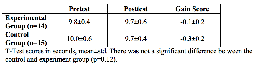
The experimental group scores were (mean±sd) pre=9.8±0.4, post=9.7±0.6, gain=-0.1±0.2. The control group scores were pre=10.0±0.6, post=9.7±0.4, gain=-0.3±0.2. The range of pre to post scores for both the experimental and control group compare favorably with and slightly faster than previously published T-Test scores for Elite U-16 soccer players (23). There was not a significant difference in gain scores between groups (p=0.12). Table 1 provides the details of the pre and posttest measures of the T-Test.

Table 1. T-Test Results

Hexagon Test
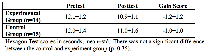
The experimental group scores were (mean±sd) pre=12.1±1.2, post=10.9±1.1, gain=-1.2±1.2. The control group scores were pre=12.0±1.4, post=11.0±1.6, gain=-1.0±1.0. The range of pre to post scores for both the experimental and control group compare favorably with and slightly faster than previously published Hexagon test scores for male recreational college athletes (4). There was not a significant difference in gain scores between groups (p=0.35). Table 2 provides the details of the pre and post measures of the Hexagon Test.

Table 2. Hexagon Test Results

20 Yard Shuttle Run
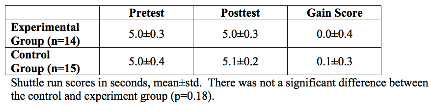
The experimental group scores were (mean±sd) pre=5.0±0.3, post=5.0±0.3, gain=0.0±0.4. The control group scores were pre=5.0±0.4, post=5.1±0.2, gain=0.1±0.3. The range of pre to post scores for both the experimental and control group compare favorably with and slightly slower than previously published 20 yard Shuttle Run Test scores for male NCAA Division III soccer athletes (23). There was not a significant difference in gain scores between groups (p=0.18). Table 3 provides the details of the pre and post measures of the 20-yard shuttle run.

Table 3. 20-Yard Shuttle Run Results

The results from all three tests indicated that there was not a significant difference at the 0.05 level in performance between the experimental and the control group. The researchers failed to reject the null hypothesis. The addition of hip rotation exercises to the training program for the experimental group did not improve performance on the agility drills versus control.

DISCUSSION
Previous research exploring means to improve agility in soccer players has focused on strength training, plyometrics, plyometrics combined with strength training, stretching modalities, and acute exercise protocols (3, 8, 9, 13, 14, 20, 22). Plyometrics, strength training, and plyometrics combined with strength training have been demonstrated to improve performance on agility tests in soccer players (9, 14, 20, 22). However, studies regarding stretching modalities (PNF, static, dynamic) and acute exercise protocols are inconclusive with respect to improving performance on agility tests (3, 8, 13). There are no other published studies investigating training of the hip rotator muscles. This study was a pioneering research experiment to determine if strengthening hip rotator muscles using latex bands could lead to improved athletic performance on agility tests. The importance of this concept brings training of hip rotator muscles into sport performance. These hip rotational exercises could be readily added to a regular strength and conditioning program.

This study introduces the concept of training hip rotator muscles into practice. By using latex chords, soccer players were able to train hip rotator musculature. In retrospect some of the players expressed feeling a difference while doing these exercises over the weeks of time. After the posttests were completed, the elastic chords were given to the Coach. The general sense from the participants was that training the hip rotator muscles was beneficial and could make a positive difference. Hence, the team continued training the hip rotator muscles with the elastic chords following the conclusion of the study. One possible reason that improvements in agility were not observed with augmented training of the hip rotator muscles was due to the large overall volume of training for both groups. The experiment was performed during the preseason transition into the regular season where training volume is high.

The researchers were unable to establish a measurable benefit from the intervention. Possibly, relative effort was related to degree of gain. Those exhibiting the greatest effort during training (from either group) experienced the greatest improvements. Some subjects may have been more motivated to work hard and win a championship, particularly the older players. Possibly, some may have trained or performed harder when influenced by a friend. The level of motivation and social acceptance may relate to work ethic. Although the research hypothesis had to be rejected, hip rotation exercises may have value in strength training programs. There may be other training programs with hip rotation exercises in favor of the research hypothesis.

The preseason workload was formidable. The beneficial expression of hip rotator supplemental exercises was possibly limited due to the large volume of other weekly exercises. If the experiment is to be repeated, one might consider the off-season when many of the variables (including total workload) can be better controlled. For example, the team could weight-train for an hour, three times per week, without the limitations of a class period (summer break). Additionally, a specific time for the experimental group to do the hip rotation exercises could be scheduled after both groups have completed the common portions of the strength training protocols together. For example, half of the players could stay after the hour-long training session for an additional 5 to 10 minutes to perform the hip rotation exercises.

A criticism of this study might focus on the repetitions and intensity in the study protocol for the hip rotator exercises. Strength protocols require higher intensity resistance with fewer repetitions whereas endurance prescribes higher repetitions with lower resistance. Arguably, the wording of the title of the study could be changed to “endurance” or “prehabilitation”. There is a relationship between muscular strength and endurance, and the small rotator muscles of the hip were isolated and exposed to focused resistance training. Nerves command muscles to pull on bones to stabilize and generate movement about joints. In theory, the nerves and motor units commanding these actions should have become stronger in response to the resistance-training stimulus. Considering the lengths, origins, and insertions, these small muscles do not create enormous amounts of torque, however, these muscles do stabilize the joint socket. The larger muscles of the legs and core move the body. The concept is to improve the stability of the joint, in turn, allowing the larger muscles to have a more stable frame to pull on. Providing the larger muscles with a more stable frame should allow for the generation of faster, more powerful movements. Further, as with the rotator cuff muscles, resistance training with high intensity and lower repetitions could be potentially hazardous to the hip rotator muscles.

Both the experimental and control groups performed total body exercises including dot drills, hang cleans, and power cleans. The dot drills, hang cleans, and power cleans were exercises where members of both groups were encouraged to move as explosively and fast as possible during the execution of the exercises while maintaining proper technique. Conversely, the tempo of the execution of the hip rotator exercises was 1:1 (seconds), with one second moving inward, followed by a one second return to the starting position for the internal hip rotation sets (with just the opposite for the external hip rotation sets). The movement speed was selected in order to strike a balance between improving the strength and stability of the joint, versus the possibility of inducing an injury to the hip rotator muscles. Ballistic movements into the limits of the range of motion may affect short or long-term risk of injury while the hip and knee are in fixed positions.

The research hypothesis was that the speed of movement and power developed as a result of performing dot drills, hang cleans, and power cleans would be better exhibited by the experimental group due to the introduction of the hip rotator exercises. The addition of hip rotator exercises was hypothesized to develop speed and power to a greater degree while performing other exercises (dot drills, hang cleans, and power cleans). Future studies might focus on the tempo of performing the hip rotator exercises. From a specificity standpoint, hip rotator exercises may need to be performed at a faster pace in order to better transfer the speed and power developed for agility performance.

CONCLUSION
In conclusion, although the research hypothesis was rejected, hip rotation exercises may still prove to be a valuable part of a strength-training program. With additional sport-related studies, the importance of hip rotation exercises augmenting a training program may prove beneficial for the enhancement of sport agility performance. These exercises may help athletes to be stronger, more agile, and less prone to injury.

APPLICATION IN SPORT
Prehabilitation is a concept where muscle groups are exposed to various exercise protocols with the hope of reducing the occurrence and severity of sport injuries (10, 11). This study could be considered prehabilitative in nature. Isolated training of the hip rotator muscles may improve the strength of the exercised muscles and enhance the long-term stability of the hip joint. Joint laxity and muscle weakness are both intrinsic risk factors for joint injury (12). A possible benefit of this study was a subsequent reduction of hip joint injuries and severity. However, the study did not include a follow up period where injury occurrences were monitored.

ACKNOWLEDGMENTS
None

REFERENCES
1. Aboodarda, S., Georg, J., Mokhtar, A., & Thompson, M. (2011). Muscle strength and damage following two modes of variable resistance training. Journal of Sports Science & Medicine, 10(4), 635-642.

2. Adkins, S. B., & Figler, R. A. (2000). Hip pain in athletes. American Family Physician, 61, 2109-2118.

3. Amiri-Khorasani, M., Sahebozamani, M., Tabrizi, K. G., & Yusof, A. B. (2010). Acute effect of different stretching methods on Illinois agility test in soccer players. Journal of Strength & Conditioning Research, 24(10), 2698-2704.

4. Baechle, T. R., & Earle, R. W. (2008). Essentials of strength training and conditioning (3rd ed.). Champaign, IL: Human Kinetics.

5. Baumgartner, T. A, & Hensley, L. D. (2006). Conducting and reading research in health and human performance (4th ed.). New York, NY: McGraw-Hill.

6. Beekhuizen, K. S., Davis, M. D., Kobler, M. J., & Cheng, M. S. (2009). Test-retest reliability and minimal detectable change of the hexagon agility test. Journal of Strength & Conditioning Research, 23(7), 2167-2171.

7. Boyd, K. T., Peirce, N. S., & Batt, M. E. (1997). Common hip injuries in sport. Sports Medicine, 24, 273-288.

8. Bullock, W., Panchuk, D., Broatch, J., Christian, R., & Stepto, N. K. (2012). An integrative test of agility, speed and skill in soccer: Effects of exercise. Journal of Science & Medicine in Sport, 15(5), 431-436.

9. Christou, M., Smilios, I., Sotiropoulos, K., Volaklis, K., Pilianidis, T., & Tokmakidis, S. P. (2006). Effects of resistance training on the physical capacities of adolescent soccer players. Journal of Strength & Conditioning Research, 20(4), 783-791.

10. Due Jakobsen, M., Sundstrup, E., Andersen, C. H., Bandholm, T., Thorborg, K., Zebis, M. K., & Andersen, L. L. (2012). Muscle activity during knee-extension strengthening exercise performed with elastic tubing and isotonic resistance. International Journal of Sports Physical Therapy, 7(6), 606-616.

11. Hamil, J., & Knutzen, K. M. (2009). Biomechanical basis of human movement (3rd ed.). Baltimore, MD: Lippincott Williams & Wilkins.

12. Jonasson, P., Halldin, K., Karlsson, J., Thoreson, O., Hvannberg, J., Swärd, L., & Baranto, A. (2011). Prevalence of joint-related pain in the extremities and spine in five groups of top athletes. Knee Surgery, Sports Traumatology, and Arthroscopy, 19(9), 1540-1546.

13. Jordan, J., Korgaokar, A. D., Farley, R. S., & Caputo, J. L. (2012). Acute effects of static and proprioceptive neuromuscular facilitation stretching on agility performance in elite youth soccer players. International Journal of Exercise Science, 5(2), 97-105.

14. Jullien, H., Bisch, C., Largouët, N., Manouvrier, C., Carling, C. J., & Amiard, V. (2008). Does a short period of lower limb strength training improve performance in field-based tests of running and agility in young professional soccer players? Journal of Strength & Conditioning Research, 22(2), 404-411.

15. Kibler, W. B. (2003). Rehabilitation of rotator cuff tendinopathy. Clinics in Sports Medicine, 22(4), 837-847.

16. Meir, R., Diesel, W., & Archer, E. (2007). Developing a prehabilitation program in a collision sport: A model developed within English premiership rugby union football. Strength & Conditioning Journal, 29(3), 50-62.

17. Mullen, G. (2010). How to prevent shoulder pain. Swimming World, 51(8), 30-31.

18. Parkkari, J. J, Kujala, U. M., & Kannus, P. P. (2001). Is it possible to prevent sports injuries? Review of controlled clinical trials and recommendations for future work. Sports Medicine, 31(14), 985-995.

19. Pauole, K. K., Madol, K. K., Garhammer, J. J., Lacourse, M. M, & Rozenek, R. (2000). Reliability and validity of the T-test as a measure of agility, leg power, and leg speed in college-aged men and women. Journal of Strength & Conditioning Research, 14(4), 443-450.

20. Ronnestad, B. R., Kvamme, N. H., Sunde, A., & Raastad, T. (2008). Short-term effects of strength and plyometric training on sprint and jump performance in professional soccer players. Journal of Strength & Conditioning Research, 22(3), 773-780.

21. Thomas, C. C., Plowman, S. A., & Looney, M. A. (2002). Reliability and validity of the anaerobic speed test and the field anaerobic shuttle test for measuring anaerobic work capacity in soccer players. Measurement in Physical Education & Exercise Science, 6(3), 187-205.

22. Thomas, K., French, D., & Hayes, P. R. (2009). The effect of two plyometric training techniques on muscular power and agility in youth soccer players. Journal of Strength & Conditioning Research, 23(1), 332-335.

23. Triplett, N. T. (2012). Speed and agility. In T. Miller (Eds.), NSCA’s guide to tests and assessments (1st ed., pp. 253-274). Champaign, IL: Human Kinetics.

U.S. Sports Academy2014-03-05T14:03:28-06:00March 5th, 2014|Contemporary Sports Issues, General, Sports Exercise Science|Comments Off

The Structure of a Team: The Influence of Goal Setting Type on Intrinsic Motivation, Group Cohesion, and Goal Achievement Orientation of Division III Female Athletes

Submitted by JoAnne Barbieri Bullard

ABSTRACT
Goal setting is found to be effective in improving group performance (20, 29). The extent to which athletes engage in goal setting and the effectiveness on mental training elements is beneficial to examine. The purpose of this study was to determine if Division III female student-athletes differed in comparison with each other regarding their previous utilization of goal setting use, to determine if goal setting type was related to intrinsic motivation based on the Sports Motivation Scale (Pelletier, Fortier, Vallerand, Tuson, Briere, & Blais, 1995), to examine if goal setting type was related to group cohesion based on the Group Environment Questionnaire (Brawley, Carron, & Widmeyer, 1987), and to examine if goal setting type was related to goal achievement orientation based on the Task Ego Orientation in Sport Questionnaire (Duda, 1989). The methodology included an informed consent form, demographics questionnaire, goal setting type measurement questionnaire, and data collection from the Sports Motivation Scale, the Group Environment Questionnaire, and the Task Ego Orientation in Sport Questionnaire. Analyses were completed utilizing bivariate correlations, Chi-square tests, and regression analysis. The results of this study supported group-focused individual goal setting was most primarily used among respondents and also resulted in significant correlations with intrinsic motivation, group cohesion, and goal achievement orientation. Athletic departments and coaching staffs can utilize these findings to coach their student-athletes most effectively.

INTRODUCTION
College athletes continually strive to enhance performance levels through numerous aspects of training. One element that has been deemed effective in enhancing performance and competitive cognitions is that of mental skills training (21, 25, 31). Goal setting is a component of mental skills training found to be effective for enhancing commitment, effort, self-confidence, and perseverance and motivation of athletes (4, 20, 26, 27) although its origins lie in organization settings (12, 15, 16, 28).

Effective goal setting is defined by who sets the goals. Self-set goals initiated by an athlete may be preferred as compared to goals set by others, including coaches and sport psychologists (33). Accepting the goals that are set is necessary for an athlete to be committed to his or her goals and positively affect performance (7, 13).

In a group setting the principles of goal setting have been shown to enhance cooperation, improve morale, and elevate collective efficacy (12). Participation in establishing group goals is correlated with improved group commitment and cohesion (28) and improved group performance with Division I student-athletes (5, 20, 24, 26, 29, 32). Individuals establishing high personal goals compatible with the goals of the group resulted in improved group performance, as compared to individual goals incompatible with the goals of the group, which diminished group performance (15).

Athletes’ intrinsic motivation, extrinsic motivation, and amotivation affect performance levels through enhancing motivation to accomplish activities, experience stimulation, and to understand a new task (8); through the use of rewards or external constraints and performing behaviors to become socially accepted and avoid negativity (8) and by experiencing feelings of incompetence and an inability to control their actions and consequences (8).

Four variables are responsible for individuals being attracted to groups including group goals, benefits of being a group member, attraction to the group due to affiliation and recognition, and comparison with other groups (17). Cohesion enhances productivity in team sports due to communication and teamwork improvement (34). Reducing the amount of motivation loss in teams enhances commitment, goal contribution, and productivity (34).

Individuals are identified according to two orientations based on their achievement abilities (18). Task orientation involves an individual establishing goals with the intention to master a skill, whereas ego orientation involves an individual feeling successful after outperforming others (18). Male and female Division III athletes with elevated levels of task orientation were more likely to have a greater sense of awareness resulting in increased performance and ability to master tasks as compared to those with elevated ego orientations (18). Ego orientated individuals had elevated levels of aggression and anxiety and lower levels of satisfaction (18). Although intrinsic motivation was related to having higher levels of task orientation, inclusion of goal setting was not found (18). It was therefore necessary to examine if Division III female athletes’ goal setting type was related to intrinsic motivation levels.

One aspect of research led to the belief that utilizing group-focused goals results in improved individual and group motivation and enhanced group performance in industrial-organizational settings (12). However, the use of group-focused individual goals within an athletic setting had not been assessed. The need to determine if goal setting type was related to student-athletes’ intrinsic motivation levels through examining the effects of previous use of goal setting is apparent.

Differences exist between athletes in their implementation of goal setting practices determining effectiveness (30). In a team atmosphere, individual athletes must work towards achieving their personal goals, as well as their team goals in order to be successful. It was possible that Division III female athletes exhibited varied goal setting type usage compared to each other.

Athletes setting team goals are found to have elevated perceptions of cohesion at the end of their season compared to the athletes who did not establish goals (24). It was thought that through having athletes develop team goals individually; each member’s feelings of involvement with the team would be enhanced (24). It was not identified if group-focused individual goal setting would impact cohesion (24). This is why it was necessary to examine if Division III female athletes’ goal setting type was related to group cohesion.

Methods
Participants
The target population of this study was Division III female student-athletes. The 76 student-athletes were members of the women’s field hockey, softball, basketball, soccer, volleyball, cross country, crew, tennis, and track and field teams. Out of the total sample size, 42 were off-season student-athletes and 34 were in-season student-athletes.

Instrumentation
Demographic information and consent. To conduct this study, each participant received an informed consent form acknowledging their volunteer participation in the study. To avoid collecting information that would identify each individual, participants were asked to report their year of education and year of participation rather than their specific age. The choices for education year included: Freshman, Sophomore, Junior, and Senior. The choices for participation year included: 1st, 2nd, 3rd, and 4th. The demographic information included: year of education; year of participation; transfer student status; sport(s) in which they participate; in-season or off-season athlete status; status as a starter or non-starter in most recent season; and individual or team sport athlete status.

Goal setting type measurement questionnaire. The three types of goal setting identified in this study were group goals, individual goals, and group-focused individual goals. In order to identify goal setting type, participants were asked to rate 18 questions (30) regarding goal setting frequency, goal setting effectiveness, goal setting effort, and goal setting barriers using a 7-point Likert scale. Participants were informed that for this study goal setting referred to the use of specific, measurable goals assisting in achieving performance measures. Overall goal frequency, overall goal effectiveness, overall goal effort, and overall ability to reach goals were also observed with this questionnaire.

Overall goal setting frequency, referring to how often participants used goal setting strategies, was assessed on responses to nine questions based on a 7-point Likert scale. Goal setting effectiveness, or the effectiveness of specific goal setting strategies, was assessed based on the responses of a 7-point Likert scale. Three questions examined overall goal setting effort based on the amount of effort participants put forth to achieve goals in specific situations and was assessed by the responses to three statements based on a 7-point Likert scale. The overall ability to reach goals was evaluated based on three questions using a 7-point Likert scale and was measured by interfering factors participants experienced.

For the purpose of this study, the goal setting type category with the highest mean value of responses was identified as the goal setting type for each student-athlete. This measurement illustrated the degree to which participants utilized or did not utilize other types of goal setting. Three questions were developed based on the definition for group goal setting, individual goal setting, and group-focused individual goal setting.

Sport Motivation Scale (SMS) (Pelletier et al., 1995). The SMS measures intrinsic motivation, extrinsic motivation, and amotivation of athletes through the use of seven subscales (10) including: intrinsic motivation to know, to accomplish things, and to experience satisfaction; extrinsic motivation of external, introjected, and identified regulation; and amotivation in reference towards sport participation (19). The SMS includes four items from each subscale totaling 28 items on the scale (11).

Participants responded to each item on a seven point Likert scale, ranging from not corresponding at all to corresponding exactly (19). An index of self-determined motivation is established after the subscales were combined (8). Athletes with high positive scores have elevated levels of sport self-determined motivation and low scores reflecting low self-determined motivation (8). Internal reliability ranged from .72 to .85 for present motivation and for perceived future motivation from .67 to .86 (19). For the purpose of this study, only intrinsic motivation from this scale was utilized to answer the 12 intrinsic motivation questions.

Group Environment Questionnaire (GEQ) (Brawley et al.,1987). The GEQ assessed perceived cohesion through the use of an 18-item, four scale instrument (3). Four components of cohesion are measured identifying a member’s attraction to the group-task (ATG-T), a member’s attraction to the group-social (ATG-S), a member’s integration into the group-task (GI-T); and a member’s integration into the group-social (GI-S) (17). Internal consistency values were r= .75, .64, .71, and .72 respectively (3). Responses for this questionnaire were based on a 9-point Likert scale (24). Nine questions referred to participants’ personal involvement with the team and nine questions referred to participants’ perceptions of their team as a whole. Participants’ scores were tallied based on each of the four variables to assess overall group cohesion. The odd numbered questions referred to the social aspects of cohesiveness, whereas the even numbered questions referred to task aspects of cohesiveness. An average was taken for each component (ATGS, GIS, ATGT, and GIT) after being summed for each participant.

Task Ego Orientation in Sport Questionnaire (TEOSQ) (Duda, 1989). The TEOSQ assessed differences in an individual’s proneness for task or ego goal orientation in athletic settings (14). This questionnaire consisted of 13 sport specific questions, which are rated on a 5-point Likert scale (18). Participants were asked to consider the phrase “I feel most successful in sport when…” prior to answering the questions (18). Overall task orientation and ego orientation resulted by averaging the total responses of each category for all participants. The TEOSQ has an alpha reliability coefficient of .62 for task orientation scale and .85 for ego orientation scale was present (9) and reported internal reliability of .80 for task orientation and .75 for ego orientation (10).

Results and Discussion
There were 76 participants of the Division III female student-athlete population (n=76). All participants received identical questionnaire packets in which they were asked to volunteer to respond to each questionnaire honestly. Two participants neglected to answer all the questions of the goal setting type measurement questionnaire, resulting in these subjects’ responses being omitted from the analyses involving these assessments. For the both the SMS and the GEQ one participant did not complete all the questions, resulting in exclusion. Four participants skipped a question on the TEOSQ, while five participants answered one question twice, resulting in the omission from this questionnaire in the data analysis (n=67). Table 1 depicts the descriptive data of the variables assessed throughout the questionnaires.

Table 1

Demographic Questionnaire
Education year and participation year. Of the 76 participants, 27.6% indicated being a freshman, 43.4% indicated being a sophomore, 17.1% indicated being a junior, and 11.8% indicated being a senior. In regard to participation year, 35.5% indicated being in their 1st year of participation, 36.8% indicated being in their 2nd year of participation, 19.7% indicated being in their 3rd year of participation, and 7.9% indicated being in their 4th year of participation.

Transfer. A total of 11 (14.5%) participants identified as being a transfer student, whereas 65 (85.5%) identified as never having transferred.

Sports. Of the student-athletes in this population, 23 identified as softball athletes, followed by 17 soccer athletes, 10 basketball athletes, nine volleyball athletes, five field hockey athletes, and three track and field athletes. Nine of the participants were dual athletes, participating in more than one sport.

Current Season. Out of the 76 participants, 44.7% identified themselves as in-season athletes, whereas 55.3% identified themselves as off-season athletes.

Starter. Out of the 76 participants, 42 (55.3%) identified as being a starter, while 34 (44.7%) identified as being a non-starter.

Sport Classification. The majority of the participants (85.5%) identified as being a team-sport athlete, whereas 14.5% identified as being an individual-sport athlete. Differences in goal setting type among individual sport athletes and team sport athletes are depicted in Table 2.

Table 2

Goal Setting Type Measurement Questionnaire
The results of this questionnaire assisted in answering if participants differed in comparison with each other regarding their previous utilization of goal setting type. Two participants were omitted from this section of the study since they did not completely answer the questionnaire, resulting in a sample of 74. The mean and standard deviation for these questions are shown in Table 1. A repeated measures ANOVA showed there was no statistically significant difference among the three goal setting types. Wilks’ Lambda = .974, F(2,27) = .98, p =.38.

Sport Motivation Scale (SMS)
The sample size for the SMS was 75 since one participant did not complete the questionnaire. Table 1 depicts participants’ mean and standard deviation results based on the average SMS scores. The three goal setting types evaluated were individual goal setting, group-focused individual goal setting, and group goal setting. A bivariate correlation analysis, depicted in Table 3, was utilized to compute the Pearson’s correlation coefficient and significance levels to measure relationships among intrinsic motivation scores and levels of each goal setting type. The total number of participants examined was 73 since three participants did not fully complete the goal setting type measurement questionnaire. The Pearson correlation calculation resulted in a positive value and relationship between SMS scores and group-focused individual goals and group goals.

Tale 3

Group Environment Questionnaire (GEQ)
Seventy-five participants completed the GEQ assessing the perceived cohesion of their teams by indicating the level of agreement with each statement. Table 1 provides the participants’ ATGS, ATGT, GIS, and GIT mean and standard deviation scores based on the GEQ. A Bivariate correlation analysis was utilized to determine the relationship among goal setting type and group cohesion variables through the use of the Pearson’s correlation coefficient and significant levels. Significant correlations at the 0.01 level (2-tailed) were found between group-focused individual goal setting and both GIT score and GIS scores. A significant correlation at the 0.05 level (2-tailed) was found between group-focused individual goal setting and ATGS score, shown in Table 4.

Table 4

Task Ego Orientation in Sport Questionnaire (TEOSQ)
The TEOSQ was utilized to assess goal orientation in an athletic environment. Participant size was limited to 67 since nine participants did not complete the questionnaires. Table 1 presents participants’ average task orientation and ego orientation mean and standard deviation scores based on the TEOSQ. A Bivariate correlation analysis was utilized to determine the relationship among goal setting type and goal orientation achievement. Through the use of the Pearson’s correlation coefficient and significance levels, the relationship was determined based on the 66 participants since one participant did not fully complete this questionnaire. The results of this analysis showed one significant positive correlation between overall task orientation and group-focused individual goal setting on the 0.01 level (2-tailed), depicted in Table 5.

Table 5

A standard regression analysis was conducted for each of the goal setting types using SMS, ego orientation, task orientation, ATGS score, ATGT score, GIS score, and GIT score as predictors, shown in Table 6. Group-focused individual goal setting was found to have the largest R squared value (.290) with SMS being the most significant predictor. Individual goal setting type was found to have the weakest positive correlation between predictor and criterion variables, shown in Table 7.

Table 6

Table 7

CONCLUSIONS
In an attempt to determine if goal setting type usage differed among respondents, the goal setting type measurement questionnaire was utilized. Respondents were found to frequently utilize all three of the goal setting types according to the overall mean scores of goal setting type use. Results indicated no difference in how frequently this sample of student-athletes used the three types of goal setting as indicated by the repeated measures ANOVA. The frequency of goal setting use among Division III female student-athletes showed that goal setting is a common practice among these athletes consistent with previous research (5, 7; 22, 29, 32, 30).

The SMS was utilized to determine if goal setting type was related to the respondents’ intrinsic motivation levels. Approximately 57.3% of the respondents’ levels of intrinsic motivation resulted above the mean score of 5.68 which was related to “corresponding a lot” in regard to intrinsic motivation based on their previous season. This supports findings regarding intrinsic motivation positively influencing participation frequency, commitment, and effort (4) in that 53% of the respondents frequently utilized goal setting practices.

Significant correlations at the 0.01 level resulted among both group-focused individual goal setting and group goal setting, whereas individual goal setting presented a weaker positive value at the 0.05 level. Respondents with elevated levels of intrinsic motivation were most likely to utilize group-focused individual goals, followed by group goals. This supported correlations between female athletes utilizing process goals and increasing motivation (26). Results indicated that goal setting type was related to this sample of athletes’ intrinsic motivation levels based on the SMS.

Respondents’ levels of cohesion were measured through the use of the GEQ to assess four variables including ATGS, ATGT, GIS, and GIT. The ATGS score, referring to respondents’ individual attractions to the group, resulted with the highest mean score. These findings support the research regarding higher levels of cohesion and involvement of groups in decision making and satisfaction (3).

ATGS score, GIS score, and GIT score were found to have a significant correlation with group-focused individual goal setting. Results indicated that group-focused individual goal setting type related to this sample of athletes’ group cohesion levels supporting previous research indicating that cohesion is found to be intricate in group goal setting and goal acceptance (3).

Athletes with high task orientation and moderate ego orientation have been found to utilize goal setting more than those with other goal orientation combinations (10). After analyzing the TEOSQ it was concluded that mean task orientation scores (4.31) were larger than mean ego orientation scores (2.71). Overall task orientation was found to have a significant correlation at the 0.01 with group-focused individual goal setting (0.346). These results showed that the respondents with higher task orientation scores had significant relationships with goal setting practices as compared to overall ego orientation scores of the respondents (9). Results indicated that group-focused individual goal setting was related to this sample of athletes’ goal achievement orientation based on the TEOSQ.

APPLICATIONS IN SPORT
This research study contributes to the field of sport psychology. The information gathered throughout this study will help athletic departments and the coaching staffs by providing information that can be utilized to assist female student-athletes with using goal setting practices beneficial for themselves and their teams. The results of this study provided insight regarding the additional variables such as intrinsic motivation, group cohesion, and goal achievement orientation that impact goal setting and may inspire future research of the impact on Division III male student-athletes and other divisions of female student-athletes. Group-focused individual goal setting was the only goal setting type significantly correlated to all three variables; intrinsic motivation, group cohesion, and goal achievement orientation. These results showed that athletes utilizing group-focused individual goals are more likely to enhance intrinsic motivation levels, group cohesion levels, and goal achievement orientation as compared to athletes utilizing individual goal setting or group goal setting practices.

ACKNOWLEDGMENTS
None

REFERENCES
1. Alexandris, K., Tsorbatzoudis, C., & Grouios, G. (2002). Perceived constraints on recreational sport participation: Investigating their relationship with intrinsic motivation, extrinsic motivation and amotivation. Journal of Leisure Research, 34(3), 233-252.

2. Brawley, L., Carron, A., & Widmeyer, W. (1987). Assessing the cohesion of teams: Validity of the group environment questionnaire. Journal of Sport Psychology, 9(3), 275-294.

3. Brawley, L., Carron, A., & Widmeyer, W. (1993). The influence of the group and its cohesiveness on perceptions of group goal-related variables. Journal of Sport & Exercise Psychology, 15(3), 245-260.

4. Burton, D., & Weiss, C. (2008). The fundamental goal concept: The path to process and performance success. In T. S. Horn, T. S. Horn (Eds.), Advances in sport psychology (3rd ed.) (pp. 339-375, 470-474). Champaign, IL US: Human Kinetics.

5. Burton, D., Weinberg, R., Yukelson, D., & Weigand, D. (1998). The goal effectiveness paradox in sport: Examining the goal practices of collegiate athletes. The Sport Psychologist, 12(4), 404-418.

6. Duda, J. L. (1989) The relationship between task and ego orientation and the perceived purpose of sport among high school athletes. Journal of Sport and Exercise Psychology, 11, 318-335.

7. Fairall, D., & Rodgers, W. (1997). The effects of goal-setting method on goal attributes in athletes: A field experiment. Journal of Sport & Exercise Psychology, 19(1), 1-16.

8. Gillet, N., Berjot, S., & Gobance, L. (2009). A motivational model of performance in the sport domain. European Journal of Sport Science, 9(3), 151-158.

9. Hanrahan, S., & Biddle, S. (2002). Measurement of achievement orientations: Psychometric measures, gender, and sport differences. European Journal of Sport Sciences, 2(5), 1-11.

10. Kim, M., Duda, J., & Gano-Overway, L. (2011). Predicting occurrence of and responses to psychological difficulties: The interplay between achievement goals, perceived ability, and motivational climates among Korean athletes. International Journal of Sport and Exercise Psychology, 9(1), 31-47.

11. Kingston, K., Horrocks, C., & Hanton, S. (2006). Do multimensional intrinsic and extrinsic motivation profiles discriminate between athlete scholarship status and gender? European Journal of Sport Science, 6(1), 53-63.

12. Kleingeld, A., Van Mierlo, H., & Arends, L. (2011). The effect of goal setting on group performance: A meta-analysis. Journal of Applied Psychology, 96(6), 1289-1304.

13. Kyllo, L., & Landers, D. (1995). Goal setting in sport and exercise: A research synthesis to resolve the controversy. Journal of Sport & Exercise Psychology, 17(2), 117-137.

14. Li, F., Harmer, P., Chi, L., & Vongjaturapat, N. (1996). Cross-cultural validation of the task and ego orientation in sport questionnaire. Journal of Sport & Exercise Psychology, 18(4), 392-407.

15. Locke, E., & Latham, G. (2006). New directions in goal-setting theory. Current Directions in Psychological Science, 15(5), 265-268.

16. Lycette, B., & Herniman, J. (2008). New goal-setting theory. Industrial Management, 50(5), 25-30.

17. Matheson, H., Mathes, S., & Murray, M. (1997). The effect of winning and losing on female interactive and coactive team cohesion. Journal of Sport Behavior, 20(3), 284-298.

18. McCarthy, J. (2011). Exploring the relationship between goal achievement orientation and mindfulness in college athletics. Journal of Clinical Sport Psychology, 5(1), 44-57.

19. Medic, N., Mack, D., Wilson, P., & Starkes, J. (2007). The effects of athletic scholarships on motivation in sport. Journal of Sport Behavior, 30(3), 292-306.

20. Mooney, R., & Mutrie, N. (2000). The effects of goal specificity and goal difficulty on the performance of badminton skills in children. Pediatric Exercise Science, 12(3), 270-283.

21. Myers, A., Whelan, J., & Murphy, S. (1996). Cognitive behavioral strategies in athletic performance enhancement. Progress in Behaviour Modification, 30, 137-164.

22. O’Brien, M., Mellalieu, S., & Hanton, S. (2009). Goal-setting effects in elite and nonelite boxers. Journal of Applied Sport Psychology, 21(3), 293-306.

23. Pelletier, L., Fortier, M., Vallerand, R., Tuson, K., Briere, N., & Blais, M. (1995). Toward a new measure of intrinsic motivation, extrinsic motivation, and amotivation in sports: The sports motivation scale (SMS). Journal of Sport & Exercise Psychology, 17(1), 35-53.

24. Senecal, J., Loughead, T., & Bloom, G. (2008). A season-long team-building intervention: Examining the effect of team goal setting on cohesion. Journal of Sport & Exercise Psychology, 30(2), 186-199.

25. Vealey, R. (1994). Current status and prominent issues in sport psychology interventions. Medicine & Science in Sports & Exercise, 26(4), 495-502.

26. Vidic, Z., & Burton, D. (2010). The roadmap: Examining the impact of a systematic goal-setting program for collegiate women’s tennis players. The Sport Psychologist, 24(4), 427-447.

27. Vosloo, J., Ostrow, A., & Watson, J. (2009). The relationships between motivational climate, goal orientations, anxiety, and self-confidence among swimmers. Journal of Sport Behavior, 32(3), 376-393.

28. Wegge, J. (2000). Participation in group goal setting: Some novel findings and a comprehensive model as a new ending to an old story. Applied Psychology: An International Review, 49(3), 498-516.

29. Weinberg, R., Burton, D., Yukelson, D., & Weigand, D. (1993). Goal setting in competitive sport: An exploratory investigation of practices of collegiate athletes. The Sport Psychologist, 7(3), 275-289.

30. Weinberg, R., Burton, D., Yukelson, D., & Weigand, D. (2000). Perceived goal setting practices of Olympic athletes: An exploratory investigation. The Sport Psychologist, 14(3), 279-295.

31. Weinberg, R., & Comar, W. (1994). The effectiveness of psychological interventions in competitive sport. Sports Medicine, 18(6), 406-418.

32. Weinberg, R., Stitcher, T., & Richardson, P. (1994). Effects of a seasonal goal-setting program on lacrosse performance. The Sport Psychologist, 8(2), 166-175.

33. Weinberg, R., & Weigand, D. (1996). Let the discussions continue: A reaction to Locke’s comments on Weinberg and Weigand. Journal of Sport & Exercise Psychology, 18(1), 89-93.

34. Williams, J., & Widmeyer (1991). The cohesion-performance outcome relationship in a coacting sport. Journal of Sport & Exercise Psychology, 13(4), 364-371.

U.S. Sports Academy2014-03-05T09:01:59-06:00March 5th, 2014|Contemporary Sports Issues|Comments Off

Leadership and Management Skills of Junior College Athletic Directors

Submitted by Timothy Baghurst, Earl Murray Jr., Chris Jayne and Danon Carter

ABSTRACT
The current and future funding condition for junior college (JC) athletics is unclear, and an athletic program’s budget and funding is usually the responsibility of the athletic director. The purpose of this qualitative phenomenological study was to explore the lived experiences and perceptions of junior college athletic directors to understand financial and leadership issues associated with athletic programs. Sixteen athletic directors (12 male, 4 female) from the same athletic conference in the state of California were interviewed and asked 17 open-ended questions about leadership and the financial issues associated with junior college athletic programs. Three primary themes emerged including leadership, roles and responsibilities, and an unexpected third theme of the student-athlete. Findings and their application to athletic director administration are discussed.

INTRODUCTION
College athletics have become big business, and a university athletic director (AD) plays an integral role in the success of the athletic programs. Colleges and universities at all levels require the managerial skills of an AD. Although leadership and administration of athletics is a frequent focus of research at the National Collegiate Athletics Association (NCAA) level, community college (hereto forth referred to as junior college; JC) programs have received little attention. For example, NCAA Division I athletic budgets may vary widely, but substantial budgets are common (14). Thus, application of findings at this level to JC athletic programs is difficult, as JC ADs may face more responsibilities in addition to fewer funding sources and athletic staff at their disposal. Therefore, the focus of this qualitative phenomenological study was to explore the lived experiences of JC ADs in order to determine how they use their leadership to overcome financial challenges experienced by their athletic programs.

Qualities of an AD
Robertson (2008) highlights several traits and skills necessary to be a successful AD. First, he or she must have the capability of creating an environment that helps all members of the program flourish, and all members of the athletic program must have the same goal in mind. Second, an AD must exhibit the ability to take risk, solve problems, think critically, and be a decision maker. Third, they must have the fiscal savvy to promote their university/college in a way that draws fan and community support thereby generating revenue. Thus, fiscal responsibilities of athletic programs are one of the most important challenges athletic administrators deal with at all levels (20).

JC Leadership Qualities
Nahavandi (2006) defined a leader as “any person who influences individuals and groups within an organization, helps them in the establishment of goals and guides them toward achievement of those goals, thereby allowing them to be effective” (p. 4). Another definition of leadership is “the capacity to influence others by unleashing their power and potential to impact the greater good” (4). Consistent with both definitions, leadership requires the ability to influence followers and guide them toward a goal.

Athletic directors are expected to display leadership skills in overseeing the day-to-day operations of the athletic department, but leadership is also necessary to manage the budget and financials of the program (13). There are several qualities of effective leadership as well as factors that impact the effectiveness of leadership. Effective leadership is defined by the effect on followers. Key traits of effective leaders as described by Kirkpatrick and Locke (1991) include drive, integrity, intelligence, motivation to lead, and knowledge of the business. Overall, leadership success is defined by the effectiveness of leaders to influence followers in every relevant aspect.

Junior college ADs must possess certain leadership qualities or characteristics to be successful. These characteristics include ethics or strong moral values, competence, self-confidence, and a desire to influence (28). Followers must trust the decisions and behaviors of ADs as well as believe in the direction being led. Leadership styles most attributed to ADs are transformational and situational leadership, as these styles incorporates change management, practicality, and flexibility as well as the success these leadership styles have on influencing others.

JC Athletic Finances
The funding for state colleges are being reduced across the country; and this is causing economic instability within many JC athletic programs (34). Junior college ADs are faced with difficult decisions when it comes to their athletic programs, which primarily revolve around the sustainability of the program. In many cases, there is outside pressure to add athletic teams to their program, while in others situations, ADs have to decide to keep a team or cut it from their program to save money (36). In 2009, Mississippi Governor Haley Barbour addressed the state’s JC ADs to explain that they needed to scale back the number of athletic teams that they offered, or the schools would have to drop athletics altogether (34).

Leadership is a key to any successful company, and sports administration is no different. However, how an AD may use his or her acquired leadership techniques to maintain and allow an athletic department to flourish under his or her guidance is unclear. This is particularly true at the JC level, where research is limited. Although there are similarities between the roles and responsibilities of ADs at JC compared with larger four-year universities, there are also differences. According to Lewis & Quarterman (2006), the three most important decisions and choices ADs make for managing and leading JC athletic programs are the enjoyment of athletics, the athletic environment, and a desire to learn more about the sports business. ADs from large universities have a greater focus on fiscal management where much of their time is focused on management, leadership, finance, marketing, ethics, legalities, and governance (2). This is not to say that JC ADs ignore ethical or legal issues, for example, but it is not considered their priority.

Although there are large financial deviations within NCAA Division I athletic programs, (14; 37), only a few operate profitably (10). Thus, the university is placed with a financial burden of justifying the existence of a program, and many DI ADs must turn to donors to gain the fiscal capital needed to balance their athletic budgets (35). For example, in the summer of 2012, facing a $4 million deficit, Maryland University decided to eliminate seven competitive athletic teams (17). Similarly, other prominent universities have taken drastic measures to ensure the survival of their athletic programs as a whole: University of California-Berkley had to cut five teams in 2010 and Rutgers University was forced to drop six competitive athletic teams in 2007 (3).

Unfortunately for ADs at the JC level, the financial situation is even bleaker. Most junior colleges lack the same opportunities. Fewer boosters are available and revenue generated at events is lower. Sustainability is a larger concern because of many educational cuts in state funding (Steinback, 2010). Success at the National Junior College Athletic Association (NJCAA) level does not always equal financial gain or even a program the next year. For example, in 2009 Minneapolis Community and Technical College lost only its second game of the year in the NJCAA DIII national championship game only to have the athletic department shut down completely shortly after. In order to continue to have an athletic program, some institutions have been required to cut the football program; although it is the biggest revenue provider, it is also the most expensive (34).

Study Purpose
The roles and responsibilities of an NCAA AD are well-documented, but less so are those of a JC AD, particularly as they pertain to leadership and financial skills. The current and future funding condition for JC athletics is unclear (6). A better understanding of the skills and qualities necessary for success could be vital as JCs search for their next AD. Therefore, the purpose of this study was to explore the perceived leadership and financial skills of 16 JC ADs to better understand how leadership and financial skills in athletic programs might contribute to success. The qualitative, phenomenological study consisted of semi-structured interviews and asked ADs not only what it was like to serve in that capacity, but also to explain, (1) the relationship between ADs’ perceptions about leadership and funding JC athletic programs, and (2) the relationship between ADs’ perceived leadership skills and financing JC athletic programs. It was intended that ADs explain in general how they perceive leadership and how it is relevant in managing programs. Then, participants were asked to detail their perceived leadership skills to manage programs effectively.

METHOD
Participants
Participants were 16 ADs (12 male, 4 female) from JCs in California who were purposefully selected because they were knowledgeable about athletic programs and financing (11). Participants’ experience ranged between 10 and 21 years (see Table 1). Currently employed ADs were used to provide real-time feedback as opposed to retroactive data.

Procedures
Following university IRB approval, 20 ADs currently employed at a JC within the same athletic conference were mailed a letter to request an interview. From the 20 requests, three participants returned the letter agreeing to participate. The remaining 17 participants were contacted by telephone from which a further 13 agreed to participate.

Prior to each interview participants were asked to sign a consent form. All face-to- face interviews lasted between 25 and 50 minutes and were conducted within a one-month period. The interviews were conducted at a neutral site of the participant’s choosing. A mini cassette recorder was used to record all interviews in their entirety. All interviews were manually transcribed by the researcher using audacity-recording software. Following transcription, each participant was sent his or her transcript to confirm its accuracy.

Instruments
In qualitative research, the researcher is the primary instrument by exploring the phenomenon under study (7). Open-ended questions navigate and focus descriptions of a particular experience through intuition and reflection of that experience. A phenomenological study requires the interviewer to achieve, or attempt to achieve, a state of epoche, the elimination of suppositions and placement of knowledge above every possible doubt (24). Thus, the primary researcher made every effort to suppress any predisposed opinions or presumptions during this study regarding the phenomenon. This allowed the researcher to grasp and freshly comprehend the participants’ experiences with the phenomenon (12).
A face-to-face interview technique with open-ended questions was the most appropriate data collection method as it allowed for some deviation while simultaneously ensuring consistent structure across interviews (12). The semi-structured, open-ended questioning interview process was designed to direct the participant toward his or her lived experiences (27).
NVivo9™ software, in accordance with the modified van Kaam data analysis method, was used to analyze interview transcripts, and identify common themes, and patterns (25). Furthermore, the software package provided a digital transcript of audio files, import, and coding of interview transcripts and aided the exploration of potential emerging themes using a step-by-step process.

Data Validity, Reliability, and Triangulation
Validity is how accurately the account represents participants’ realities of the phenomenon and their credibility (16). To establish the validity for this study, transcripts were shared with the participants to ensure that the data was accurate prior to analysis, which is an important dimension of good quality research (9). This allowed participant to edit, revise, or add information prior to data analysis, none of which did. If both validity and reliability are the goal of qualitative research, the use of triangulation to record the construction of reality is appropriate (18). Triangulation occurs when different data sources, methods of data collection, or types of data are evidence to support research data (12). In the present study, participants were sent interview transcripts and themes derived from the data to ensure its accuracy as a second data source as well as confirm thematic analysis.

Data Analysis
According to Bradley, Curry, and Devers (2007), there is no singular way to conduct qualitative data analysis, although there is general agreement that the process is ongoing. An important first step is to immerse and comprehend the meaning (5). A modification of the van Kaam method of analysis for phenomenological data, which occurs through a multi-step process, was employed in the present study (24). This method identifies common themes and patterns used by participants in a qualitative research study.

The first step requires data to be organized, transcribed, and coded. Organization of data is critical in qualitative research because of the large amount of information gathered during the study (12). The data was organized by material type: all interviews, all observations, and all documents. Finally, data was coded.

The next step in the modified van Kaam data analysis method requires participants’ statements to be categorized, clustered, coded, and labeled into groups (24). The common themes constituting the core elements of the lived experiences of the participants were most important. Coding is a process of making sense of the data, dividing the data into text or image segments, labeling the segments with codes, examining codes for overlap and redundancy, and collapsing these codes into broad themes (12).

RESULTS
The premise of this study was to develop an understanding about the leadership skills of ADs with a particular focus on financial expertise. A semi-structured interview process was used to develop an overall analysis of expert thinking. The analysis revealed three emerging themes: (a) leadership, (b) roles and responsibilities, and (c) student-athletes. Each theme is explained and then supported by participant quotes.

Theme One: Leadership
With respect to leadership, leadership skills, types, and supervision were considered important. Participants mentioned the skills to self-evaluate and feedback and how important it was to reflect on their own performances. Self-evaluation is necessary in addition to soliciting feedback from others who might be able to provide insight. Participant 1 said,

I think through and self-evaluate, and each year I am evaluated by the Vice President and President of the college. The evaluation process also includes coaches, the trainer, and the secretary to find out what I need to improve on and set some goals.

Participant 12 stated, “Understanding my leadership skills involves listening to feedback and asking questions about how I am doing. A good leader must be open to constructive criticism and be a good listener and respect others’ opinions.”

The leadership of ADs may also influence the success of programs. According to Participant 6,

I am a leader by example as a positive person. I am reasonable and approachable, and [I] motivate with pride. I am a leader who likes to inspire others to be better. I am successful if our programs are. I want my coaches and student-athletes to be successful. I want to get the most out of people and care about what they are doing as followers.

Furthermore, Participant 3 said that

As a transformational leader, I look at the goals and vision of the athletic department and what needs to be done for the long term. Each athletic program has different needs and I look at the short and long term goals.

Theme Two: Roles and Responsibilities
A JC AD has multiple roles and responsibilities, but balancing budgets, securing funding, and distributing it appropriately was mentioned frequently. This is supported by Participant 6 who stated that, “Overseeing the budgets is a big part of my job. We have so much money for each program. Every program has a different number of student-athletes, coaches, etc. Each budget is different.”

Athletic directors must be able to budget well for each program they oversee. This is a challenge, as they must find ways to generate revenue to keep the programs active. For example, Participant 7 referred to fundraising.

Fundraising is the best way. I do not know of a community college that does not
fundraise. Most institutions cannot provide things such as backpacks or gear. There are strict rules about what can be purchased with state or district dollars. When there is a shortfall of funds, we have to fundraise to support the programs.

Participant 16 found that securing the necessary budget for JC athletics is frequently a challenge.

Money is very tight for athletic programs at community colleges. As a staff, we must fundraise to keep the programs going. The coaches fundraise for their sport. Some fundraising activities may be charity golf tournaments, barbeques, or bake sales.

Although finances are just one component of the responsibilities of an AD, it is apparent that they are a significant concern. For example, according to Participant 14, “The budget consumes 70% of my time to ensure the programs are run effectively.”

The decisions about athletic programs are a major responsibility for ADs. Participants reported that Title IX Gender Equity was a concern when adding, removing, or maintaining a program. “Title IX gender equity and compliance is a big issue, and we have to evaluate our athletic programs when considering adding or dropping a program”, said Participant 9. Participant 15, who stated that decisions about programs were made in consideration of Title IX and gender equity, supported this. Thus, it becomes a balancing act of meeting guidelines or policies while simultaneously ensuring that there is a sufficient budget.

I try to keep all my athletic programs. I try to make sure they are maintained with enough dollars coming in to keep them going. Terminating a program is the last thing I try to do. If nothing else, adding a program is a good thing but that takes money.

(Participant 16)

In JC athletics, things can change quickly, an AD must make decisions concerning their coaching staff who are responsible for the student-athlete. Thus, a change in a staff member may directly impact the athletic program and the student-athletes. According to Participant 4,
In athletics, change happens often. I deal with change by telling my coaches about changes and we work together on making changes when the time comes. Some people resist change, but change is a reality in athletics.

It is important, therefore, for the AD to be cognizant of upcoming change, and keep the staff apprised of changes that might impact them.

My coaches must deal with change the most because they spend the most time with the student-athletes. I teach them about change, when change is going to take place, how it affect their programs, and help them with change. Some adapt to change well, and others do not. I work with them all.

(Participant 8)

Theme Three: Student-Athletes
Some ADs reported the additional responsibility of having to coach. Although an AD wants to win both as a coach and director, there is recognition of balancing athletic success with academic success. In fact, the ADs placed academics above athletics. According to Participant 16, “The student-athlete should manage time by first looking at their academic responsibilities first then sports.” This is further supported by other examples.

The balance is placing academics ahead of athletics. The student-athlete must be organized and set up time schedules. A balanced student-athlete focuses toward academics and although athletics is important, earning good grades is equally important.

(Participant 14)

Athletic directors recognize that academic success is a reflection on the future prospects of the student-athlete, but also on the JC. Transferring to a larger institution is important for many students.

A student-athlete who cares about moving on beyond a two year college will do a good job with balancing academics and athletics. Although the student-athlete can do well in a sport, the student must have a good grade point average to transfer.

(Participant 8)

Motivation plays a big role in the student-athlete performance athletically and academically. The ADs are tasked with working with coaches to assist with motivating athletes. Just as a coach is a mentor to an athlete, the AD must serve as a mentor to the coach. According to Participant 13, “The athletic director sets the stage for the coaches to motivate the student-athletes.”

I try to promote morale and motivation with my coaches who are the leaders for the student-athlete. The coaches are mentors who motivate and inspire the student-athlete to good. As the athletic director I train the coaches to engage the student-athlete.

(Participant 2)

Some student-athletes are less self-motivated than others and require external motivation to perform better in a sport or academics. The ability to prioritize athletics and completing coursework with passing grades can be a challenge, yet “Increasing his or her self-motivation in the classroom can lead to a successful student-athlete” (Participant 11). Participant 6 noted that athletics has a tendency to be placed ahead of academics.

The challenged student-athlete lacks self-motivation, direction, and the ability to manage their time. This type of student-athlete lacks the passion for being engaged academically to learn in the classroom. They place athletics ahead of academics, which may be why they have difficulties earning good grades in the classroom.

DISCUSSION
The purpose of this qualitative, phenomenological study was to explore ADs lived experiences and perceptions of leadership in JC athletic programs particularly in reference to finances. Interview analysis revealed three main themes of leadership, roles and responsibilities, and the student-athlete. Each theme is discussed in light of current research.

Theme One: Leadership
Athletic directors recognized the importance of leadership in influencing the behavior and actions of others. According to Smith (1997), “As leaders face greater uncertainties and changes, and compounded complexities, they strive for greater flexibility and agility” (p. 277). In the present study, ADs saw their role as leaders encompassing a variety of roles and responsibilities as evidenced in the second theme. What is most important with these varying roles and responsibilities is the opportunity to receive feedback on their performance and make the appropriate adjustments based on the feedback received. “Effective leaders learn that comprehensive systematic reviews and evaluations should include every type of resource, every competency and capacity, and every person and position that affects performance” (33). Thus, some participants acquired evaluations from superiors, such as the college president or those working for the participant such as coaches, and applied this feedback to improve their leadership styles and effectiveness. Overall, the feedback an AD receives is a measuring tool for effectiveness in their role.

Theme Two: Roles and Responsibilities
Balancing budgets and securing funding was a clear concern for the participants. Many participants indicated that they were responsible for preparing the budget. A participative budget process involves lower-level administrators and coaches who better understand the individual line items who are responsible for the athletic department’s budget than senior administrators. A top down budgeting process offers short-term budgets imposed by senior administrators more likely to be consistent with the strategic long-term goals and objectives of the athletic department (20). Thus, those ADs expected to complete budgets without the use of participative budget methodology may experience higher levels of stress (32). Participative budgeting is supported by Wickstrom (2006), as an authoritative style of leadership is not conducive to the work force of the modern era, and that to be a successful leader an AD has to be willing to listen to those they lead.

The present study further found that gender equity and the budgetary requirements that stem from Title IX was considered both a financial and leadership challenge. This is not surprising, as gender equity at JCs has been clearly documented (8). A balance needs to exist between athletic sports programs relative to women’s sports and Title IX laws (19). Some ADs are faced with the decision to cut sports programs (Steinback, 2010) and must be cognizant of their current Title IX standing so that there does not become an imbalance of participation opportunities. Thus, there remains work to be done in achieving a standard of gender equity that not only meets the intent of Title IX but fully affords the respect of dignity for female student-athletes (19). As two-year athletic programs consider new directions, the achievement of gender equity within two year athletic programs still needs to be addressed (19), which is recognized by the participants of the present study.
Theme Three: Student-Athletes
The relationship that ADs had with student-athletes was an unexpected finding. This may be in part because some ADs reported the additional responsibility of serving as a coach. The extra coaching duties may cause additional stressors because it limits the time they have to devote to the financial responsibilities of the profession (21). Participants recognized that they were responsible with the coaches for improving both student athletic and academic performance. Participants stressed the importance of academics over athletics, but this may be due to efforts by the administration to increase retention and graduation rates (29). Not only did ADs report high levels of interaction with student-athletes, they generally viewed it as part of their responsibility to motivate the student to achieve both in athletics and in the classroom. That ADs viewed this as a component of their leadership was unexpected, as this task is frequently the responsibility of a coach or even assistant (15).

Limitations and Future Research
Although the present study provides some interesting findings, they should be evaluated with respect to its limitations. First, this study was limited to current full-time ADs at JCs in the state of California, which may not translate to the experiences of ADs in other locations or athletic conferences. Second, only four participants were female. This is not uncommon (1), and future research should consider whether opinions and perceptions differ between genders. For example, impressions of Title IX may differ by gender (1), and Title IX challenges may differ between JCs and traditional four-year institutions. Third, the specific financial expertise of each participant was not assessed. Therefore, future research should consider whether financial education and training improves AD financial expertise and progress toward short, intermediate, and long term strategic goals. The recommendation may benefit both low-level and senior level administrators at the JC. In addition, future researchers should consider conducting a broader survey of the general background and experiences of ADs in JCs.

CONCLUSIONS
The success of collegiate athletic programs can depend upon the skills of their ADs (31). Thus, they must possess leadership skills across multiple disciplines. Because financial and budgetary concerns were most prevalent among the participants of the present study, future research needs to investigate the training being provided for ADs. The financing and budget process is vital in ensuring that athletic programs are successful, and an action plan is needed for current and future ADs to use as a model to understand the entire financial and budget process of funding athletics programs.

APPLICATIONS IN SPORT
Empirical research has focused primarily on the Division I AD. However, these findings suggest that JC ADs encounter a variety of challenges which have not been investigated. JC administrators need to consider the budgetary and fundraising background and expertise of applicants, which is a paramount responsibility of ADs in JC.

ACKNOWLEDGMENTS
None
REFERENCES
1. Anderson, D. J., Cheslock, J. J., & Ehrenberg, R. G. (2006). Gender equity in intercollegiate athletics: Determinants of Title IX compliance Journal of Higher Education, 77, 225-250.

2. Barr, C. A., Hums, M. A., & Masteralexis, L. P. (2009). Principles and practice of sport management (3rd ed.). Sudbury, MA: Jones and Bartlett.

3. Berkowitz, S. (2011, June 28). Rutgers athletic department needs fees, funds to stay afloat. USA Today. Retrieved from http://usatoday30.usatoday.com/sports/college/2011-06-28-rutgers-athletic-department-subsidies_n.htm

4. Blanchard, K. (2010). Leading at a higher level: Blanchard on leadership and creating high performing organizations. Upper Saddle River, NJ: BMC, Blanchard Management Corporation.

5. Bradley, E. H., Curry, L. A., & Devers, K. J. (2007). Qualitative data analysis for health services research: Developing taxonomy, themes, and theory. Health Services Research, 42, 1758-1772.

6. Byrd, L. A., & Williams, M. R. (2007). Expansion of community college athletic programs. Community College Enterprise, 13, 39-49.

7. Caldwell, L., Creswell, J., & Iwamoto, D. K. (2007). Feeling the beat: The meaning of rap music for ethnically diverse Midwestern college students: A phenomenological study. Adolescence, 42, 337-351.

8. Castaneda, C., Hardy, D. E., & Kastinas, S. G. (2008). Meeting the challenge of gender equity in community college athletics. New Directions for Community Colleges, 142, 93-105.

9. Cohen, D., J., & Crabtree, B. F. (2008). Evaluation criteria for qualitative research in health care: Controversies and recommendations. Animals of Family Medicine, 6, 331-339.

10. Cooper, C., & Weight, E. (2011). Investigating NCAA administrator values in NCAA Division I athletic departments. Journal of Issues in Intercollegiate Athletics, 4, 74-89.

11. Creswell, J. W. (1994). Research design: Qualitative and quantitative approaches (1st ed.). Thousand Oaks, CA: Sage Publications, Inc.

12. Creswell, J. W. (2005). Educational research: Planning, conducting, and evaluating quantitative and qualitative research. (2nd ed.). Upper Saddle River, NJ: Pearson.

13. Davis, D. J. (2001). An analysis of the perceived leadership styles and levels of satisfaction of selected junior college athletic directors and head coaches. United States Sports Academy. Retrieved from Proquest, UMI Dissertations Publishing, 3026212.

14. Dunn, J. M. (2013). Should the playing field be leveled? Funding inequities among Division I athletic programs. Journal of Intercollegiate Sport, 6, 44-51.

15. Fitzgerald, M. P., Nelson, B., & Sagaria, M. D. (1994). Career patterns of athletic directors: Challenging the conventional wisdom. Journal of Sport Management, 8, 14-26.

16. Ferguson, L. (2004). External validity, generalizability, and knowledge utilization. Journal of Nursing Scholarship, 36, 16-22.

17. Giannotto, M. (2012, July 2). Maryland cuts seven sports on ‘sad day’ in College Park, Washington Post. Retrieved from http://articles.washingtonpost.com/2012-07-02/sports/35486395_1_athletic-programs-track-program-athletic-director-kevin-anderson

18. Golafshani, N. (2003). Understanding reliability and validity in qualitative research. Qualitative Report, 8, 597-607.

19. Hagedorn, L. S., & Horton D., Jr. (2009). Student athletes and athletics. New Directions for Community Colleges, 147, 1-91.

20. Hodge, F., & Tanlu, L. (2009). Finances and college athletics. New Directions for Institutional Research, 140, 7-18.

21. Judge, L. W., & Judge, I. L. (2009). Understanding the occupational stress of interscholastic athletic directors. ICHPER – SD Journal of Research in Health, Physical Education, Recreation, Sport & Dance, 4, 37-44.

22. Kirkpatrick, S. A., & Locke, E. A. (1991). Leadership: Do traits matter? Executive, 5, 48-60.

23. Lewis, B. A., & Quarterman, J. (2006). Why students return for a master’s degree in sport management. College Student Journal, 40, 717-728.

24. Moustakas, C. (1994). Phenomenological research methods. Thousand Oakes, CA: Sage Publications.

25. Mukamusoni, D. (2006). Distance learning program of teachers at Kigali institute of education: An expository study. International Review of Research in Open and Distance Learning, 3, 1-10.

26. Nahavandi, A. (2006). The art and science of leadership. Upper Saddle River, NJ: Pearson. Prentice Hall.

27. Nelson, B., & Rawlings, D. (2007). Its own reward: A phenomenological study of artistic creativity. Journal of Phenomenological Psychology, 38, 217-255.

28. Northouse, P. G. (2013). Leadership: Theory and practice. Thousand Oaks, CA: SAGE.

29. Ohlson, M., & Storch, J. (2009). Student services and student athletes in community colleges. New Directions for Community Colleges, 147, 75-84.

30. Robertson, J. E. (2008). Leadership, athletic directors and mental toughness. National Junior College Athletic Association Review, 60, 2-6.

31. Ruihley, B. J., & Fall, L. T. (2009). Assessment on and off the field: Examining athletic directors’ perceptions of public relations in college athletics. International Journal of Sport Communication, 2, 398-410.

32. Ryska, T. A. (2002). Leadership styles and occupational stress among college athletic directors: The moderating effect of program goals. Journal of Psychology, 136, 1-22.

33. Smith, A. W. (1997). Leadership is a living system: Learning leaders and organizations. Human Systems Management, 16, 277-284. Retrieved from ProQuest at http://search.proquest.ezproxy.apollolibrary.com/docview201129759?

34. Steinbach, P. (2010). Economic Storm. National Junior College Athletic Association Review, 62, 4-7.

35. Wickstrom, B. D. (2006). Message to ADs: Get to know donors. National Collegiate Athletic Association News, 43, 4-24.

36. Williams, M. R., Byrd, L., & Pennington, K. (2008). Intercollegiate athletics at the community college. Community College Journal of Research and Practice, 32, 453-461.

37. Zimbalist, A. (2013). Inequality in intercollegiate athletics: Origins, trends and policies. Journal of Intercollegiate Sport, 6, 5-24.

U.S. Sports Academy2014-03-06T15:54:25-06:00March 3rd, 2014|Contemporary Sports Issues, General, Sports Management, Sports Studies and Sports Psychology|Comments Off

Correlates of Performance at the USRowing Youth National Championships: A Case Study of 152 Junior Rowers

Submitted by Alex Wolff & Pavle Mikulic

ABSTRACT
This study was designed to assess the extent of the relationship between a number of variables (2000 m rowing ergometer score, weight adjusted 2000 m rowing ergometer score, height, weight, and years of experience) and placement at the USRowing Youth National Championships, in order to highlight areas for college recruiters and aspiring junior rowers to focus on. Data for 152 athletes competing in 18 events was collected. Data collection was accomplished through a site search of “berecruited.com” for the keywords “youth nationals” “nationals” and “rowing”; athletes reported placement was then verified against the official race results. Athletes were subdivided into categories based on boat size, event type, weight class, and gender. In almost all categories (with the exception of men’s open weight sweep and lightweight sculls) a significant (p<0.05) correlation between rowing ergometer score and placement was established. The highest correlation between rowing ergometer score and placement was observed in women’s lightweight sculls (r=0.76). Weight adjustment provided notable improvements in only two categories over unadjusted ergometer score: men’s open weight sculls (r=0.79 vs. r=0.72) and men’s lightweight sculls (r=0.49 vs. r=0.42). Weight independent of ergometer score and experience did not correlate with final rankings. Height independent of ergometer score correlated with final rankings in only one category - men’s open sculls (r=0.38). While it is possible that the small sample sizes in some categories may have impacted the results, a clear trend emerges emphasizing the importance of unadjusted rowing ergometer score over other factors in evaluating junior rowers at the national level.

INTRODUCTION
Rowing is a strength-endurance activity that requires both aerobic and anaerobic capability for successful performance (Maestu, Jurimae, & Jurimae, 2005; Secher, 2000). A typical rowing race takes place over a 2000 m course and, depending on the boat category and weather conditions, is characterized by 5.5 – 7.5 minutes of exhaustive physical effort. Rowing comprises two distinct, but closely related disciplines: sculling and sweep rowing. The main distinction between the two is that sculling involves the use of two oars per rower, one in each hand, versus only one slightly larger oar for sweep rowers. Of the two, sculling is considered more technically demanding, and sweep is more popular, particularly at the collegiate level where major sculling regattas are largely nonexistent. All rowing boats can also be divided into two additional categories: small boats (boats with one or two crew members, i.e. single sculls, double sculls and pairs) and large boats (boats with four or eight rowers, i.e. quadruple sculls, coxed and coxless fours and eights). Typically, the larger the boat is, the more stable it becomes because of the additional hull width and length. Because of this, a single can be a much different boat to row than an eight. Additionally, larger boats increase the importance of synchronization of crew members’ strokes to achieve increased speed (Baudouin & Hawkins, 2002). A more recent addition to the world of competitive rowing has been the advent of lightweight events. USRowing defines lightweight junior rowers as weighing no more than 160 or 130 pounds for men and women, respectively. Lightweight events at Youth National Championships are lightweight double, lightweight four, and lightweight eight.

Besides its international popularity as a competitive sport and its continuous presence on Olympic Games from the very first modern Olympic Games held in 1896 in Athens, Greece, rowing is also a major collegiate sport in various countries, including the United States. With this in mind, it may be of particular interest for college recruiters to gain a better understanding of the factors that contribute to rowing performance in junior rowers competing at the most important event at the national level: the USRowing Youth National Championships. Likewise, it may be important for prospective junior rowers and their coaches to be able to focus on those factors which contribute to greater on-water performance.

College recruiters are continuously striving to improve the selection process for their rowing teams and, when assessing a junior rower’s ability, they can be presented with a wide array of factors to consider. With this in mind, we designed this study to assess the strength of association between a number of objective variables and race placement at the USRowing Youth National Championships. The variables we examined include years of experience, body height, body weight, 2000 m rowing ergometer score and 2000 m weight adjusted rowing ergometer score. Based on our two earlier studies (Mikulic et al. 2009a,b) in which we observed a strong correlation between 2000 m rowing ergometer performance scores and final rankings at both World Rowing Championships and World Junior Rowing Championships, we hypothesized that 2000 m rowing ergometer score (an “all-out” effort over a distance of 2000 m) would be the strongest correlate to placement at the USRowing Youth National Championships. However, the extent to which this is true and the relation of other variables to rowing performance in junior rowers competing at the USRowing Youth National Championships has yet to be determined.

METHODS
The data for this study was collected by performing a site search of athlete’s profiles on the “berecruited.com” web site. This site allows athletes to upload their information such as personal best 2000 m ergometer score along with other facts such as their height, weight, and notable race results, all in an effort to increase their visibility to college recruiters. We performed the search using the keywords “youth nationals” “nationals” and “rowing”. Those profiles which listed a 2012 or 2013 Youth Nationals result were then matched to the official race results from their respective year to verify that athletes reported placement. Once verified, that athlete’s information and placement was included in the data set. The variables recorded were: 2000 m rowing ergometer score (personal best), height, weight, years of experience, and weight adjusted 2000 m ergometer score based on the following formula (6):

Adjusted ergometer score = (rower weight/270)^0.22* ergometer score in seconds

The data was then divided into a number of sub categories which were as follows: open weight overall, open category scull and open category sweep. Rowers were further classified as open category men, open category women, lightweight men, and lightweight women. The correlation between each factor and placement was established for each category using the Pearson product moment correlation coefficient. The significance of correlation coefficients was tested to a confidence of p=0.05. In addition, we performed a series of independent samples t-tests to examine the differences in rowing ergometer scores between selected groups of rowers.

RESULTS
Tables 1 and 2 indicate that 2000 m ergometer scores, both in absolute values and adjusted to a rower’s weight, demonstrate the most consistent association with final rankings at the USRowing Youth Championships. This is especially evident in women’s events in which the correlations between the ergometer scores and final rankings were evident in all of the observed categories (i.e. scull and sweep, open category and lightweight rowers).

Table 1. Correlation coefficients between final rankings at the USRowing Youth Championships and five observed variables in groups of male junior rowers

Table 2. Correlation coefficients between final rankings at the USRowing Youth Championships and five observed variables in groups of female junior rowers

T-tests were utilized to test for differences in ergometer scores between sweep oar rowers and scullers (Table 3). The only category in which a significant difference was observed between scullers and sweep oar rowers was the men’s lightweight category. There was no significant difference between women’s lightweight sweep oar rowers and scullers, women’s open category sweep oar rowers and scullers, or men’s open category sweep oar rowers and scullers. Similarly, when ergometer scores of big vs. small boat rowers were compared, no significant differences were observed across the categories except for the men’s lightweight category (Table 4).

Table 3. 2000-m Rowing ergometer scores (in seconds) for various categories of rowers and independent samples t-test results for differences between sweep oar rowers vs. scullers

Table 4. 2000 m Rowing ergometer scores (in seconds) for various categories of rowers and independent samples t-test results for differences between rowers in small vs. big boats

DISCUSSION
In this study we aimed to identify the variables that showed the strongest association with the final rankings at the most important competition for junior rowers in the US – the USRowing Youth Championships. The results (Tables 1 and 2) indicate that 2000 m rowing ergometer scores, both in absolute values and adjusted to body weight, displayed the strongest correlations across categories, both for junior men and women. In junior men, the strongest correlations were observed for open category sculling events (r=0.72 for ergometer score; r=0.79 for weight adjusted ergometer score) while in junior women the strongest correlation were observed for lightweight category sculling events (r=0.76 for both ergometer score and weight adjusted ergometer score). These findings largely corroborate findings from our earlier study (Mikulic et al. 2009a) in which we observed moderate to high correlation coefficients between 2000 m rowing ergometer score and final rankings at the World Rowing Junior Championships. In that study, rowing ergometer scores of junior rowers correlated with their final rankings in all 13 events in which the junior rowers competed at the 2007 World Rowing Junior Championships with the correlation coefficient ranging from r=0.31 to r=0.92.

Weight adjusted rowing ergometer scores are ergometer scores normalized to that specific rowers speed in an eight boat. Since heavier rowers sink the boat further into the water, thus creating more wetted surface and drag, they must be capable of producing greater power to achieve the same speed as a lighter rower. This should, in theory, improve upon the correlation produced by non-weight-adjusted scores which we failed to observe on a consistent basis in the present study (Tables 1 and 2). The categories for which weight adjustment provided the largest improvement (men’s open and lightweight sculls) had comparatively small standard deviations versus other groups. It is possible that weight adjustment thus becomes more of a factor since the difference in “raw power” (represented by the ergometer score) between rowers was not as exaggerated as other categories for which weight adjustment provided no improvement.

Experience, height and weight of junior rowers did not generally correlate with final rankings at the USRowing Youth Championships, with the exception of height which correlated with the final rankings in junior men’s open category sculling events (r=-0.38), and experience which correlated with final rankings in junior women’s open category sculling events (r=-0.52). This general lack of association between the body size variables (i.e. height and weight) and final rankings at the Championships is somewhat surprising given the well documented importance of body size for rowing performance (for a review, see Shephard, 1998) including rowing performance at the junior level (Burgois 2000; 2001). It is possible that since Youth Nationals is a lower level of competition than junior worlds, the regatta analyzed in the studies cited, the larger variance in skill and general fitness (and, by extension, the ergometer score) would outweigh the importance of body size.

There appear to be no differences in 2000 m rowing ergometer scores of junior male and female rowers who compete in sculling vs. sweep rowing events (Table 3). The exception are junior men’s lightweight categories in which scullers are about 10 seconds faster than their counterparts from sweep rowing boats. Similarly, 2000 m rowing ergometer scores of junior men and women do not appear to differ for those competing in big vs. the small boats. Again, the only exception are junior lightweight categories in which rowers competing in a small boat are about 10 seconds faster than their counterparts competing in a big boat. Apparently, 2000 m ergometer score does not appear to be a factor for selecting a junior rower to a sculling vs. the sweep boat or the big vs. the small boat. In our earlier study (Mikulic et al., 2009a) we also observed no differences between 2000 m ergometer scores of scullers and sweep rowers competing at the 2007 World Junior Championship, either for male or female rowers (no rowers compete in lightweight categories at World Junior Championships). However, in that study, we also observed that better 2000 m ergometer performers tended to be selected to large boats. We must, however, mention a limitation of comparing 2000 m ergometer scores of various groups of junior rowers in this study as the numbers of rowers in comparing groups differed substantially thus reducing the accuracy of t-test analyses.

CONCLUSIONS
In conclusion, the most important factor to consider in the recruitment of junior rowers is rowing ergometer score over 2000 meters. This finding largely confirmed our original hypothesis. In certain categories (particularly men’s open weight categories), weight adjusting provided some improvements and may be useful in distinguishing between candidates with similar ergometer scores. Years of experience, height, and weight independent of ergometer score were shown to have very little correlation with actual boat speed.

APPLICATIONS IN SPORT
When evaluating junior rowers as potential candidates for recruitment, the most important factor appears to be the 2000 m rowing ergometer score. While weight adjustment can in certain scenarios aid in evaluation, it is only marginally effective at best. Experience, height, and weight should be largely ignored as these factors have very little impact on boat speed. Junior rowers looking to perform well at Youth National Championships should focus their efforts on improving their 2000 m rowing ergometer scores.

ACKNOWLEDGMENTS
None

REFERENCES
1. Baudouin, A., & D. Hawkins. (2002). A biomechanical review of factors affecting rowing performance. British Journal of Sports Medicine, 36(6), 396-402.

2. Maestu, J., Jurimae, J., & Jurimae, T. (2005). Monitoring of performance and training in rowing. Sports Medicine, 35, 597–617.

3. Secher, N. H. (2000). Rowing. In R. J. Shephard & P. O. A°strand (Eds.), Endurance in sport (pp. 836–843). Oxford: Blackwell Science.

4. Mikulic, P., Smoljanovic, T., Bojanic, I., Hannafin, J., Pedisic, Z. (2009a). Does 2000-m rowing ergometer performance time correlate with final rankings at the World Junior Rowing Championship? A case study of 398 elite junior rowers. Journal of Sports Sciences, 27(4), 361–366.

5. Mikulic, P., Smoljanovic, T., Bojanic, I., Hannafin, J.A., Matkovic, B.R. (2009b). Relationship between 2000-m rowing ergometer performance times and World Rowing Championships rankings in elite-standard rowers. Journal of Sports Sciences, 27(9), 907–913.

6. Weight Adjustment Calculator. (n.d.). Home. Retrieved November 23, 2013, from http://www.concept2.com/indoor-rowers/training/calculators/weight-adjustment-calculator

7. Bourgois, J., Claessens, A.L., Vrijens, J., Philippaerts, R., Van Renterghem, B., Thomis, M. et al. (2000). Anthropometric characteristics of elite male junior rowers. British Journal of Sports Medicine, 34, 213-216.

8. Bourgois J, Claessens AL, Janssens M, Van Renterghem B, Loos R, Thomis M, Philippaerts R, Lefevre J, Vrijens J. (2001). Anthropometric characteristics of elite female junior rowers. Journal of Sports Sciences, 19(3), 195-202.

9. Shephard, R.J. (1998). Science and medicine of rowing: a review. Journal of Sports Sciences, 16, 603-620.

U.S. Sports Academy2016-04-01T09:27:20-05:00March 3rd, 2014|Contemporary Sports Issues, Sports Exercise Science, Sports Studies and Sports Psychology|Comments Off

Factors Affecting Scoring in NFL Games and Beating the Over/Under Line

Submitted by C. Barry Pfitzner, Steven D. Lang and Tracy D. Rishel

ABSTRACT
In this paper we attempt to predict the total points scored in National Football League (NFL) games for the 2010-2011 season. Separate regression equations are identified for predicting points for the home and away teams in individual games based on information known prior to the games. The sum of the predictions for the home and away teams computed from the regression equations (updated weekly) are then compared to the over/under line on individual NFL games in a wagering experiment to determine if a successful betting strategy can be identified. All predictions in this paper are out-of-sample—meaning that all of the information necessary for the predictions was available before the games were played. Using this methodology, we find that several successful wagering strategies could have been applied to the 2010-2011 NFL season. We also estimate a single equation to predict the over/under line for individual games. That is, we test to see if the variables we have collected and formulated are important in predicting the betting line for NFL games. These results can be used by either bettors or bookmakers wanting to increase their odds of success in the gaming industry.

INTRODUCTION
Bookmakers set over/under lines for virtually all NFL games. Suppose the over/under line for total points in a particular game is 40. Suppose further that a gambler wagers with the bookmaker that the actual points scored in the game will exceed 40, that is, he bets the “over.” If the teams then score more than 40 points, the gambler wins the wager. If the teams score under 40 points, the gambler loses the bet. If the teams score exactly 40 points, the wager is tied and no money changes hands. The process works symmetrically for bets that the teams will score fewer than 40 points, or betting the “under.” The over/under line differs, of course, on individual games. Since losing bets pay a premium (often called the “vigorish,” “vig,” or “juice” and typically equal 10%), the bookmakers will profit as long the money bet on the “over” is approximately equal to the amount of money bet on the “under” (bookmakers also sometimes “take a position,” that is, they will welcome unbalanced bets from the public if the bookmaker has strong feelings regarding the outcome of the wager [see also the reference to Levitt’s work in the literature review]). It is widely known a gambler must win 52.4% of the wagers to be successful. That particular calculation can be established simply. Let Pw = the proportion of winning bets and (1 – Pw ) = the proportion of losing bets. The equation for breaking even on such bets where every winning wager nets $10 and each losing wager represents a loss of $11 is:
Pw ($10) = (1 – Pw ) ($11) , and solving for Pw
Pw = 11∕21 = .5238, or approximately 52.4%

This research attempts to identify methods of predicting the total points scored in a particular game based on information available prior to that game. The primary research question is whether or not these methods can then be utilized to formulate a successful gambling strategy for the over/under wager, with success requiring a winning percentage of at least 52.4%.

The remainder of this paper is organized as follows: in the next section we describe the efficient markets hypothesis as it applies to the NFL wagering market; we then offer a brief review of the literature; in the following section we describe the data and method; descriptive statistics and the main regression results are then presented; these are followed by the wagering simulations; we next discuss our investigation of the determinants of the over/under line; and finally offer our conclusions.

NFL Betting as a Test of the Efficient Markets Hypothesis
A number of important papers have treated wagering on NFL games as a test of the Efficient Market Hypothesis (EMH). This hypothesis has been widely studied in economics and finance, often with focus on either stock prices or foreign exchange markets. Because of the difficulties of capturing EMH conclusions given the complexities of those markets, some researchers have turned to the simpler betting markets, including sports (and the NFL), as a vehicle for such tests.

If the EMH holds, asset prices are formed on the basis of all information. If true, then the historical time series of such asset prices would not provide information that would allow investors to outperform the naïve strategy of buy-and-hold (see, for example, Vergin 2001). As applied to NFL betting, if the use of past performance information on NFL teams cannot generate a betting strategy that would exceed the 52.4% win criterion, the EMH hypothesis holds for this market. Thus, the thrust of much of the research on the NFL has taken the form of attempts to find winning betting strategies, that is, strategies that violate the weak form of the EMH.

A Brief Review of the Recent Literature
Nearly all of the extant literature on NFL betting uses the point “spread” as the wager of interest. The spread is the number of points by which one team (the favorite) is favored over the opponent (the underdog). Suppose team A is favored over team B by 7 points. A wager on team A is successful only if team A wins by more than 7 points (also known as “covering” the spread). Symmetrically, a wager on team B is successful only if team B loses by fewer than 7 points or, of course, team B wins or ties the game—in any of these cases, team B “covers.” Vergin (2001) and Gray and Gray (1997) are examples of research that focus on the spread.

Based on NFL games from 1976 to 1994, Gray and Gray (1997) find some evidence that the betting spread is not an unbiased predictor of the actual point spread on NFL games. They argue that the spread underestimates home team advantage, and overstates the favorite’s advantage. They further find that teams who have performed well against the spread in recent games are less likely to cover in the current game, and those teams that have performed poorly in recent games against the spread are more likely to cover in the current game. Further Gray and Gray find that teams with better season-long win percentages versus the spread (at a given point in the season) are more likely to beat the spread in the current game. In general, they conclude that bettors value current information too highly, and conversely place too little value on longer term performance. That conclusion is congruent with some stock market momentum/contrarian views on stock performance. Gray and Gray then use the information to generate probit regression models to predict the probability that a team will cover the spread. Gray and Gray find several strategies that would beat the 52.4% win percentage in out-of-sample experiments (along with some inconsistencies). They also point out that some of the advantages in wagering strategies tend to dissipate over time.

Vergin (2001), using data from the 1981-1995 seasons, considers 11 different betting strategies based on presumed bettor overreaction to the most recent performance and outstanding positive performance. He finds that bettors do indeed overreact to outstanding positive performance and recent information, but that bettors do not overreact to outstanding negative performance. Vergin suggests that bettors can use such information to their advantage in making wagers, but warns that the market and therefore this pattern may not hold for the future.

A paper by Paul and Weinbach (2002) is a departure from the analysis of the spread in NFL games. They (as do we in this paper) target the over/under wager, constructing simple betting rules in a search for profitable methods. These authors posit that rooting for high scores is more attractive than rooting for low scores. Ceteris paribus, then, bettors would be more likely to choose “over” bets. Paul and Weinbach show that from 1979-2000, the under bet won 51% of all games. When the over/under line was high (exceeded the mean), the under bet won with increasing frequency. For example, when the line exceeded 47.5 points, the under bet was successful in 58.7% of the games. This result can be interpreted as a violation of the EMH at least with respect to the over/under line.

Levitt (of Freakonomics fame) approaches the efficiency question from a different perspective. It is clear that if NFL bets are balanced, the bookmaker will profit by collecting $11 for each $10 paid out. As we suggested earlier, bookmakers at times take a “position” on unbalanced bets, on the assumption that the bookmaker knows more about a particular wager than the bettors. Levitt presents evidence that the spread on games is not set according to market efficiency. For example, using data from the 2001-2002 seasons, he shows that home underdogs beat the spread in 58% of the games, and twice as much was bet on the visiting favorites. Bookmakers did not “move the line” to balance these bets, thus increasing their profits as the visiting favorite failed to cover in 58% of the cases.

Dare and Holland (2004) re-specify work by Dare and MacDonald (1996) and Gray and Gray (1997) and find no evidence of the momentum effect suggested by Gray and Gray, and some, but less, evidence of the home underdog bias that has been consistently pointed out as a violation of the EMH. Dare and Holland ultimately conclude that the bias they find is too small to reject a null hypothesis of efficient markets, and also that the bias may be too small to exploit in a gambling framework.

Still more recently, Borghesi (2007) analyzes NFL spreads in terms of game day weather conditions. He finds that game day temperatures affect performance, especially for home teams playing in the coldest temperatures. These teams outperform expectations in part because the opponents were adversely acclimatized (for example, a warm weather team visiting a cold weather team). Borghesi shows this bias persists even after controlling for the home underdog advantage.

METHODS
We focus on the total points scored in NFL games and the corresponding over/under line for that game. With the objective of estimating regression equations for home and away team scoring, data were gathered for the 2010-11 season for the analysis. The variables include:
TP = total points scored for the home and visiting teams for each game played
PO = passing offense in yards per game
RO = rushing offense in yards per game
PD = passing defense in yards per game
RD = rushing defense in yards per game
GA = “give aways,” offensive turnovers per game
TA = “take aways,” defensive turnovers per game
D = a dummy variable equal to 1 if the game is played in a closed dome, 0 otherwise
PP = points scored by a given team in their prior game
L = the over/under betting line on the game

Match-ups Matter (we think)
The general regression format is based on the assumption that “match ups” are important in determining points scored in individual games. For example, if team “A” with the best passing offense is playing team “B” with the worst passing defense, ceteris paribus, team “A” would be expected to score many points. Similarly, a team with a very good rushing defense would be expected to allow relatively few points to a team with a poor rushing offense. In accord with this rationale, we formed the following variables:
PY = PO + PD = passing yards
RY = RO + RD = rushing yards

For example, suppose team “A” is averaging 325 yards (that’s high) per game in passing offense and is playing team “B” which is giving up 330 yards (also, of course, high) per game in passing defense. The total of 655 would predict many passing yards will be gained by team “A,” and likely many points will be scored by team “A.”

Similarly, we theorize that if a team’s offense that commits many turnovers plays a team whose defense causes many turnovers, points scored for the offensive team may be lower (and perhaps more points will be scored by the defensive team). For turnovers, we created variables similar to the passing and rushing yards in the previous paragraph:
TO = GA + TA, that is, turnovers = “give aways” for a given team plus “take aways” for the opposition team.
The dome variable will be a check to see if teams score more (or fewer) points if the game is played indoors.
The variable for points scored in the prior game (PP) is intended to check for streakiness in scoring. That is, if a team scores many (or few) points in a given game, are they likely to have a similar performance in the ensuing game?

We also test to ascertain whether or not scoring is contagious. That is, if a given team scores many (or few) points, is the other team likely to score many (or few) points as well? We test for this by two-stage least squares regressions in which the predicted points scored by each team serve as explanatory variables in the companion equation.

General Regression Equations
The general sets of regressions attempted are of the form:
where the subscripts h and v refer to the home and visiting teams respectively, and the i subscript indicates a particular game.

Equations such as 1 and 2 are estimated using data for weeks 5 through 17 of the 2010-11 season. We chose to wait until week five to begin the estimations so that statistics on offense, defense, turnovers, etc., are more reliable than would be the case for earlier weeks.

RESULTS AND DISCUSSION
Descriptive Statistics
Table I contains some summary statistics for the data set. Teams averaged approximately 223 yards passing per game (offense or defense, of course) for the season, and they averaged approximately 115 yards rushing. The statistics reported on the rushing and passing standard deviations without parentheses are for the offenses and the defensive standard deviations are (as you might guess) in parentheses. Interestingly, passing defense is less variable across teams than is passing offense (we hypothesize that teams must be more balanced on defense to keep other teams from exploiting an obvious defensive weakness, but teams may be relatively unbalanced offensively and still be successful [see the 2011 Packers, for example, who ranked near the top in passing offense and near the bottom in rushing defense]). Home teams scored approximately 23.2 points on average for the season and outscored the visitors by 1.7 points. Total points averaged 44.5 in 2010-2011 and the over/under line averaged 42.8 (the difference between these means is statistically significant at α < .10; the calculated value for the t-test of paired samples is approximately 1.92). Not surprisingly, the standard deviation was much smaller for the line than for total points. Table I: Summary Statistics

Regression Results
Though equations 1 and 2 from above represent our theoretical foundation, we did not find empirical support for the dome effect, points scored in the prior game, or for turnovers in predicting points for either the home or away teams. Thus we do not report regressions with those variables included (such estimations are available from the authors upon request). Since our objective is to produce predictions based on variables (and their effects) that are known prior to the games, we updated the equations weekly and checked for effects for those excluded variables. We did not find convincing evidence that any of the excluded variables should be included in the predictive equations.

The dome effect in a previous paper (see Pfitzner, Lang, & Rishel, 2009) found that teams scored approximately 5.4 more points when the game was played in a closed dome stadium for the 2005-2006 season. However, for the 2010-2011 season, games played in domes averaged 45.4 points and games played outdoors averaged 44.3. That difference is not statistically significant; the t-test for independent samples yields a calculated value of 0.54. The dome effect may be idiosyncratic in that, in some seasons, the high scoring teams may happen to be those who play home games in domed stadiums.

The representative estimated equations (at the end of the 16th week) are given in Table II. For the home points equation, the passing yardage and the rushing yardage are significant at α < .01, and α < .05 levels, respectively. The equation explains a modest 4.2% ( ) of the variance in home points scored. On the other hand, the F-statistic indicates that the overall equation meets the test of significance at α < .01. The estimated coefficients for the variables have the anticipated signs. To interpret those coefficients, an additional 100 yards passing (recall that this is the sum of the home team’s passing offense and the visitor’s passing defense) implies approximately 4.3 additional points for the home team, whereas an additional 100 yards rushing implies approximately 4.2 additional points. Table II: Regression Results for Total Points Scored

The visiting team estimation yields a similar equation in terms of the overall fit. The explanatory variables are statistically significant—the passing yardage variable at α < .05, and the rushing yardage variable is significant at α < .01. The equation explains only 3.7% ( ) of the variance in visiting team points, and the F-statistic implies overall significance at α < .05. The coefficients perhaps suggest a more important role for rushing than for passing in scoring for the visiting team. If the coefficients are to be believed, an additional 100 yards passing yields approximately 2.8 points for the visiting team, and an additional 100 yards rushing is worth 6.7 points. The reader may find such low values to be of concern, but recognize that the variables for which we are attempting estimates are very difficult to predict and are subject to wide variation. As we show in a later section, the lines on the games are much easier to predict. The model is best judged by its prediction qualities—here based on wagering success. Other Hypotheses
Another hypothesis we wished to entertain is whether or not scoring is contagious. A priori, we surmised that points scored in given games for visiting and home teams would be positively related. In keeping with our earlier work, there is no evidence that such is the case. The estimated simple correlation coefficient between home team and visiting team points is -0.106, which is not statistically different from zero and “wrong” signed according to our intuition. Our initial thinking was that if team “A” scores and perhaps takes a lead, team “B” has greater incentive to score. An obvious complicating factor is that a given team may dominate time of possession, thus preventing the opposing team opportunities to score. We also experimented with two-stage least squares to test the hypotheses that scoring was contagious. In that formulation we developed a “predicted points” variable for the home team, entered that variable as an independent variable in the visiting team equation, and reversed the procedure for the home team equation. Neither of the predicted points variables were statistically significant. The variable was positively signed for the home team equation, and negatively signed for the away team equation.

As indicated above, we also find no evidence that teams are “streaky” with respect to points scored. In short, we find that points scored in the immediately prior week do not contribute to the explanation of points scored in the current week. That conclusion holds up for the regressions in section VI as well.
Finally, though turnovers clearly matter in who wins or loses, there is no evidence from our work that measuring teams’ turnovers per game prior to the current game aids in predicting points scored by the individual teams.

Wagering on the Over/Under Line
In this simulated wagering project we use the estimated equations to predict scores of the home and away teams for all of the games played over weeks 8 through week 17 (end of the regular season). The points predicted in this manner are then compared to the over/under line for each game. We then simulate betting strategies on those games.

Out-of-Sample Method
Since it is widely known that betting strategies that yield profitable results “in sample,” are often failures in “out-of-sample” simulations, we use a sequentially updating regression technique for each week of games. Suppose, for example, we are predicting points for week 8. We then estimate equations TPhi and TPvi with the data from weeks 5, 6, and 7, then “feed” those equations with the known data for each game through the end of week 7, generating predicted points for the visiting and home team for all individual games in week 8. The predicted points are then totaled and compared to the over/under line for each game. Next we add the data from week 8, re-estimate equations TPhi and TPvi, and make predictions for week 9. The same updating procedure is then used to generate predictions for weeks 10 through 17. This method ensures that our results are not tainted with in-sample bias.

Betting Strategies
We entertain three betting strategies for the predicted points versus the over/under line on the games. These strategies are:
1. Bet only games for which our predicted total points differ from the line by more than 7 points.
2. Bet only games for which our predicted total points differ from the line by more than 5 points.
3. Bet all games for which our predicted total points differ from the line by any amount—in our case, all games.

As stated previously, a betting strategy on such games must predict correctly at least 52.4% of the time to be successful. If a given method cannot beat this 52.4% criterion, as a betting strategy it is deemed to be a failure.

Table III contains a summary of the results for the three betting strategies. The first betting strategy yields only ten “plays” over weeks 6 to 17. That betting strategy would have produced five wins, and five losses. For this (very) small sample, this strategy is, of course, not profitable, with only a 50% winning percentage. The second strategy (a differential greater than 5 points) yields 39 plays and a record of 17-10-0—a winning percentage of 63%. Finally for every game played, the method produces a still profitable record of 97-78-5, with the winning percentage at 55.4%.

Table III: Results of Different Betting Strategies

There is some consistency between these results and those we found for the 2005-2006 season. In that work we found that the “> 5 points” strategy produced a winning percentage of 60.5% based on 39 plays. Betting all games produced a winning percentage of 54%. Interestingly, the earlier research produced nine games with a greater than 10 point difference between the line and the predicted points whereas this work on 2010-2011 season produced only one play (which would have been a winning bet).

It is important to note that we make no adjustment for injuries, weather, and the like that would be considered by those who make other than simulated wagers. We offer these methods only as a guide, not as a final strategy.

Another Method of Predicting the Line and Total Points
Since we have collected and created variables that may be relevant to determining the betting line (and total points), in this section we investigate the relevancy of our variables in that context. For purposes of comparison, we estimate an equation for the over/under line and, separately, for the actual points scored. Further, we compare the results for the 2010-11 season with our results from prior research. These equations may be useful in confirming (or contradicting) the results of the previous sections, and may provide useful information applicable to wagering strategies.

The results of those regressions are contained in Table IV. We estimated regression equations for two seasons with the line as the dependent variable and all of the right-hand side variables (with the exception of turnovers) specified in equations 1 and 2. The estimations for the line are contained in the second column (2005-2006 season) and the fourth column (2010-2011 season). The estimations are remarkably similar. For the line for both seasons, every coefficient estimate is correctly signed and statistically significant at traditional levels of alpha, and for both equations. The line seems to be set on the assumption that teams are streaky (we conclude they are not), and the dome effect on the betting line seems to be a bit smaller in the most recent season.

Table IV: Regression Results for the Line and Total Points, 2005 and 2010 Seasons

As a comparison, we also estimated (far less successfully) an equation for total points with the same set of explanatory variables with those results reported in columns three and five of Table IV. Perhaps the most striking result of these regressions is that the regressions for the line explain fully two-thirds of the variance in that dependent variable and the equations for the actual points explains less than 6% of the variance in total points for either season, with only four of the seven explanatory variables meeting the test for statistical significance at traditional levels for 2005-2006 and only three for 2010-2011. Interestingly, the dome effect for total points for the earlier season estimated 5 additional points scored in dome games, and the corresponding estimate for the 2010-11 season was zero, when controlling for other effects. Recall that for the 2005-2006 season, 5.4 points more were scored in games played in domes, and the corresponding difference was only one point for the 2010-2011 season.

In short, and to be expected, the line is much easier to predict than is actual points scored. That is, the outcome of the games and points scored therein are not easily predicted. It is tempting to say, “That’s why they play the games.” At least two further observations are in order. First, consider the coefficients for points scored in the previous game. Those variables matter as would be anticipated on an a priori basis in determining the line for the game. However, they seem to play an insignificant (statistical or practical) role determining the actual points scored. This particular result may be interpreted as bettors placing too much emphasis on recent information, as other authors have suggested.

Finally, it also seems clear that the effect of playing indoors has dissipated between the two seasons for which we report results in Table IV. As we have emphasized, this may be simply the effect of teams who play many games indoors having poorer scoring teams for any particular year.

CONCLUSIONS
The regression results in this paper identify promising estimating equations for points scored by the home and away teams in individual games based on information known prior to the games. In a regression framework, we apply the model to three simulated betting procedures for NFL games during weeks 6 through 17 of the 2010-2011 season. Betting strategies based on the differences between our predictions and the over/under line produced profitable results for either all games at any differential or those for which our predictions differed from the betting line by 5 or more points.

Based on our earlier results finding profitable wagering strategies for the 2005-2006 season, we (and others) questioned whether these results will hold up in other seasons. Based on the results presented here—so far, so good.

APPLICATIONS IN SPORT
Betting on sports, the NFL in particular, is a very popular pastime among sports (or gambling) enthusiasts and a very lucrative business for bookmakers in Las Vegas and elsewhere. This research was conducted to determine whether successful wagering strategies could be developed based on regression equations used to predict points for the home and away teams in individual games. The sum of the predictions for the home and away teams, updated weekly, were then compared to the over/under line on individual NFL games. Certain betting strategies were identified as successful, and could therefore be used by those wanting to improve their odds while enjoying and increasing their interest in America’s favorite sport.

ACKNOWLEDGMENTS
None

REFERENCES
1. Badarinathi, R., & Kochman, L. (2001). Football betting and the efficient market hypothesis. The American Economist, 40(2), 52-55.

2. Borghesi, R. (2007). The home team weather advantage and biases in the NFL betting market. Journal of Economics and Business, 59, 340-354.

3. Boulier, B. L., Steckler, H. O., & Amundson, S. (2006). Testing the efficiency of the National Football League betting market. Applied Economics, 38, 279-284.

4. Dare, W. H., & Holland, A. S. (2004). Efficiency in the NFL betting market: modifying and consolidating research methods. Applied Economics, 36, 9-15.

5. Dare, W. H., & MacDonald, S. S. (1996). A generalized model for testing home and favourite team advantage in point spread markets. Journal of Financial Economics, 40, 295-318.

6. Gray, P. K., & Gray, S. F. (1997). Testing market efficiency: Evidence from the NFL sports betting market. The Journal of Finance, LII(4), 1725-1737.

7. Levitt, S. D. (2002). How do markets function? An empirical analysis of gambling on the National Football League. National Bureau of Economic Research (Working Paper No. 9422).
8. Paul, R. J., & Weinbach, A. P. (2002). Market efficiency and a profitable betting rule: Evidence from totals on professional football. Journal of Sports Economics, 3, 256-263.

9. Pfitzner, C. B., Lang, S. D., & Rishel, T. D. (2009). The determinants of scoring in NFL games and beating the over/under ;ine. New York Economic Review, 40, 28-39.

10. Pfitzner, C. B., Lang, S. D., & Rishel, T. D. (2006). Can regression help to predict total points scored in NFL games? In A. Avery (Ed.), The 2006 Southeastern INFORMS Conference Proceedings (pp. 312-317). Myrtle Beach, SC: Southeastern INFORMS.

11. Vergin, R. C. (2001). Overreaction in the NFL point spread market. Applied Financial Economics, 11, 497-509.