The United States Sports Academy is an independent, non-profit, accredited sports university created to serve the nation and the world with programs in instruction, research, and service. The role of the Academy is to prepare our men and women for careers in the profession of sports using modern technologies and traditional teaching methodologies.
ABSTRACT This study was designed to assess the extent of the relationship between a number of variables (2000 m rowing ergometer score, weight adjusted 2000 m rowing ergometer score, height, weight, and years of experience) and placement at the USRowing Youth National Championships, in order to highlight areas for college recruiters and aspiring junior rowers to focus on. Data for 152 athletes competing in 18 events was collected. Data collection was accomplished through a site search of “berecruited.com” for the keywords “youth nationals” “nationals” and “rowing”; athletes reported placement was then verified against the official race results. Athletes were subdivided into categories based on boat size, event type, weight class, and gender. In almost all categories (with the exception of men’s open weight sweep and lightweight sculls) a significant (p<0.05) correlation between rowing ergometer score and placement was established. The highest correlation between rowing ergometer score and placement was observed in women’s lightweight sculls (r=0.76). Weight adjustment provided notable improvements in only two categories over unadjusted ergometer score: men’s open weight sculls (r=0.79 vs. r=0.72) and men’s lightweight sculls (r=0.49 vs. r=0.42). Weight independent of ergometer score and experience did not correlate with final rankings. Height independent of ergometer score correlated with final rankings in only one category - men’s open sculls (r=0.38). While it is possible that the small sample sizes in some categories may have impacted the results, a clear trend emerges emphasizing the importance of unadjusted rowing ergometer score over other factors in evaluating junior rowers at the national level.
INTRODUCTION Rowing is a strength-endurance activity that requires both aerobic and anaerobic capability for successful performance (Maestu, Jurimae, & Jurimae, 2005; Secher, 2000). A typical rowing race takes place over a 2000 m course and, depending on the boat category and weather conditions, is characterized by 5.5 – 7.5 minutes of exhaustive physical effort. Rowing comprises two distinct, but closely related disciplines: sculling and sweep rowing. The main distinction between the two is that sculling involves the use of two oars per rower, one in each hand, versus only one slightly larger oar for sweep rowers. Of the two, sculling is considered more technically demanding, and sweep is more popular, particularly at the collegiate level where major sculling regattas are largely nonexistent. All rowing boats can also be divided into two additional categories: small boats (boats with one or two crew members, i.e. single sculls, double sculls and pairs) and large boats (boats with four or eight rowers, i.e. quadruple sculls, coxed and coxless fours and eights). Typically, the larger the boat is, the more stable it becomes because of the additional hull width and length. Because of this, a single can be a much different boat to row than an eight. Additionally, larger boats increase the importance of synchronization of crew members’ strokes to achieve increased speed (Baudouin & Hawkins, 2002). A more recent addition to the world of competitive rowing has been the advent of lightweight events. USRowing defines lightweight junior rowers as weighing no more than 160 or 130 pounds for men and women, respectively. Lightweight events at Youth National Championships are lightweight double, lightweight four, and lightweight eight.
Besides its international popularity as a competitive sport and its continuous presence on Olympic Games from the very first modern Olympic Games held in 1896 in Athens, Greece, rowing is also a major collegiate sport in various countries, including the United States. With this in mind, it may be of particular interest for college recruiters to gain a better understanding of the factors that contribute to rowing performance in junior rowers competing at the most important event at the national level: the USRowing Youth National Championships. Likewise, it may be important for prospective junior rowers and their coaches to be able to focus on those factors which contribute to greater on-water performance.
College recruiters are continuously striving to improve the selection process for their rowing teams and, when assessing a junior rower’s ability, they can be presented with a wide array of factors to consider. With this in mind, we designed this study to assess the strength of association between a number of objective variables and race placement at the USRowing Youth National Championships. The variables we examined include years of experience, body height, body weight, 2000 m rowing ergometer score and 2000 m weight adjusted rowing ergometer score. Based on our two earlier studies (Mikulic et al. 2009a,b) in which we observed a strong correlation between 2000 m rowing ergometer performance scores and final rankings at both World Rowing Championships and World Junior Rowing Championships, we hypothesized that 2000 m rowing ergometer score (an “all-out” effort over a distance of 2000 m) would be the strongest correlate to placement at the USRowing Youth National Championships. However, the extent to which this is true and the relation of other variables to rowing performance in junior rowers competing at the USRowing Youth National Championships has yet to be determined.
METHODS The data for this study was collected by performing a site search of athlete’s profiles on the “berecruited.com” web site. This site allows athletes to upload their information such as personal best 2000 m ergometer score along with other facts such as their height, weight, and notable race results, all in an effort to increase their visibility to college recruiters. We performed the search using the keywords “youth nationals” “nationals” and “rowing”. Those profiles which listed a 2012 or 2013 Youth Nationals result were then matched to the official race results from their respective year to verify that athletes reported placement. Once verified, that athlete’s information and placement was included in the data set. The variables recorded were: 2000 m rowing ergometer score (personal best), height, weight, years of experience, and weight adjusted 2000 m ergometer score based on the following formula (6):
Adjusted ergometer score = (rower weight/270)^0.22* ergometer score in seconds
The data was then divided into a number of sub categories which were as follows: open weight overall, open category scull and open category sweep. Rowers were further classified as open category men, open category women, lightweight men, and lightweight women. The correlation between each factor and placement was established for each category using the Pearson product moment correlation coefficient. The significance of correlation coefficients was tested to a confidence of p=0.05. In addition, we performed a series of independent samples t-tests to examine the differences in rowing ergometer scores between selected groups of rowers.
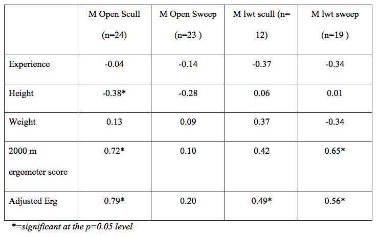
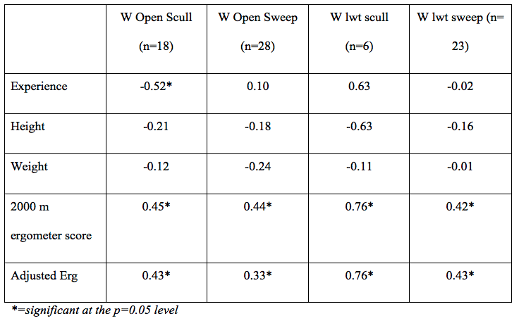
RESULTS Tables 1 and 2 indicate that 2000 m ergometer scores, both in absolute values and adjusted to a rower’s weight, demonstrate the most consistent association with final rankings at the USRowing Youth Championships. This is especially evident in women’s events in which the correlations between the ergometer scores and final rankings were evident in all of the observed categories (i.e. scull and sweep, open category and lightweight rowers).
Table 1. Correlation coefficients between final rankings at the USRowing Youth Championships and five observed variables in groups of male junior rowers
Table 2. Correlation coefficients between final rankings at the USRowing Youth Championships and five observed variables in groups of female junior rowers
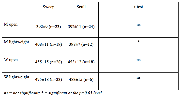
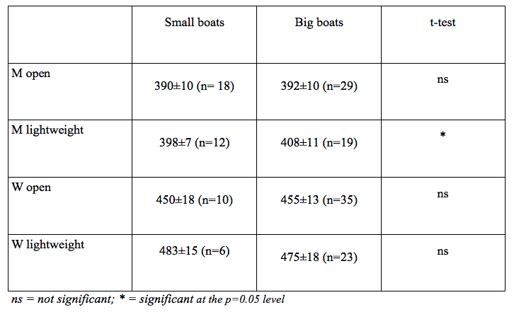
T-tests were utilized to test for differences in ergometer scores between sweep oar rowers and scullers (Table 3). The only category in which a significant difference was observed between scullers and sweep oar rowers was the men’s lightweight category. There was no significant difference between women’s lightweight sweep oar rowers and scullers, women’s open category sweep oar rowers and scullers, or men’s open category sweep oar rowers and scullers. Similarly, when ergometer scores of big vs. small boat rowers were compared, no significant differences were observed across the categories except for the men’s lightweight category (Table 4).
Table 3. 2000-m Rowing ergometer scores (in seconds) for various categories of rowers and independent samples t-test results for differences between sweep oar rowers vs. scullers
Table 4. 2000 m Rowing ergometer scores (in seconds) for various categories of rowers and independent samples t-test results for differences between rowers in small vs. big boats
DISCUSSION In this study we aimed to identify the variables that showed the strongest association with the final rankings at the most important competition for junior rowers in the US – the USRowing Youth Championships. The results (Tables 1 and 2) indicate that 2000 m rowing ergometer scores, both in absolute values and adjusted to body weight, displayed the strongest correlations across categories, both for junior men and women. In junior men, the strongest correlations were observed for open category sculling events (r=0.72 for ergometer score; r=0.79 for weight adjusted ergometer score) while in junior women the strongest correlation were observed for lightweight category sculling events (r=0.76 for both ergometer score and weight adjusted ergometer score). These findings largely corroborate findings from our earlier study (Mikulic et al. 2009a) in which we observed moderate to high correlation coefficients between 2000 m rowing ergometer score and final rankings at the World Rowing Junior Championships. In that study, rowing ergometer scores of junior rowers correlated with their final rankings in all 13 events in which the junior rowers competed at the 2007 World Rowing Junior Championships with the correlation coefficient ranging from r=0.31 to r=0.92.
Weight adjusted rowing ergometer scores are ergometer scores normalized to that specific rowers speed in an eight boat. Since heavier rowers sink the boat further into the water, thus creating more wetted surface and drag, they must be capable of producing greater power to achieve the same speed as a lighter rower. This should, in theory, improve upon the correlation produced by non-weight-adjusted scores which we failed to observe on a consistent basis in the present study (Tables 1 and 2). The categories for which weight adjustment provided the largest improvement (men’s open and lightweight sculls) had comparatively small standard deviations versus other groups. It is possible that weight adjustment thus becomes more of a factor since the difference in “raw power” (represented by the ergometer score) between rowers was not as exaggerated as other categories for which weight adjustment provided no improvement.
Experience, height and weight of junior rowers did not generally correlate with final rankings at the USRowing Youth Championships, with the exception of height which correlated with the final rankings in junior men’s open category sculling events (r=-0.38), and experience which correlated with final rankings in junior women’s open category sculling events (r=-0.52). This general lack of association between the body size variables (i.e. height and weight) and final rankings at the Championships is somewhat surprising given the well documented importance of body size for rowing performance (for a review, see Shephard, 1998) including rowing performance at the junior level (Burgois 2000; 2001). It is possible that since Youth Nationals is a lower level of competition than junior worlds, the regatta analyzed in the studies cited, the larger variance in skill and general fitness (and, by extension, the ergometer score) would outweigh the importance of body size.
There appear to be no differences in 2000 m rowing ergometer scores of junior male and female rowers who compete in sculling vs. sweep rowing events (Table 3). The exception are junior men’s lightweight categories in which scullers are about 10 seconds faster than their counterparts from sweep rowing boats. Similarly, 2000 m rowing ergometer scores of junior men and women do not appear to differ for those competing in big vs. the small boats. Again, the only exception are junior lightweight categories in which rowers competing in a small boat are about 10 seconds faster than their counterparts competing in a big boat. Apparently, 2000 m ergometer score does not appear to be a factor for selecting a junior rower to a sculling vs. the sweep boat or the big vs. the small boat. In our earlier study (Mikulic et al., 2009a) we also observed no differences between 2000 m ergometer scores of scullers and sweep rowers competing at the 2007 World Junior Championship, either for male or female rowers (no rowers compete in lightweight categories at World Junior Championships). However, in that study, we also observed that better 2000 m ergometer performers tended to be selected to large boats. We must, however, mention a limitation of comparing 2000 m ergometer scores of various groups of junior rowers in this study as the numbers of rowers in comparing groups differed substantially thus reducing the accuracy of t-test analyses.
CONCLUSIONS In conclusion, the most important factor to consider in the recruitment of junior rowers is rowing ergometer score over 2000 meters. This finding largely confirmed our original hypothesis. In certain categories (particularly men’s open weight categories), weight adjusting provided some improvements and may be useful in distinguishing between candidates with similar ergometer scores. Years of experience, height, and weight independent of ergometer score were shown to have very little correlation with actual boat speed.
APPLICATIONS IN SPORT When evaluating junior rowers as potential candidates for recruitment, the most important factor appears to be the 2000 m rowing ergometer score. While weight adjustment can in certain scenarios aid in evaluation, it is only marginally effective at best. Experience, height, and weight should be largely ignored as these factors have very little impact on boat speed. Junior rowers looking to perform well at Youth National Championships should focus their efforts on improving their 2000 m rowing ergometer scores.
ACKNOWLEDGMENTS None
REFERENCES 1. Baudouin, A., & D. Hawkins. (2002). A biomechanical review of factors affecting rowing performance. British Journal of Sports Medicine, 36(6), 396-402.
2. Maestu, J., Jurimae, J., & Jurimae, T. (2005). Monitoring of performance and training in rowing. Sports Medicine, 35, 597–617.
3. Secher, N. H. (2000). Rowing. In R. J. Shephard & P. O. A°strand (Eds.), Endurance in sport (pp. 836–843). Oxford: Blackwell Science.
4. Mikulic, P., Smoljanovic, T., Bojanic, I., Hannafin, J., Pedisic, Z. (2009a). Does 2000-m rowing ergometer performance time correlate with final rankings at the World Junior Rowing Championship? A case study of 398 elite junior rowers. Journal of Sports Sciences, 27(4), 361–366.
5. Mikulic, P., Smoljanovic, T., Bojanic, I., Hannafin, J.A., Matkovic, B.R. (2009b). Relationship between 2000-m rowing ergometer performance times and World Rowing Championships rankings in elite-standard rowers. Journal of Sports Sciences, 27(9), 907–913.
6. Weight Adjustment Calculator. (n.d.). Home. Retrieved November 23, 2013, from http://www.concept2.com/indoor-rowers/training/calculators/weight-adjustment-calculator
7. Bourgois, J., Claessens, A.L., Vrijens, J., Philippaerts, R., Van Renterghem, B., Thomis, M. et al. (2000). Anthropometric characteristics of elite male junior rowers. British Journal of Sports Medicine, 34, 213-216.
8. Bourgois J, Claessens AL, Janssens M, Van Renterghem B, Loos R, Thomis M, Philippaerts R, Lefevre J, Vrijens J. (2001). Anthropometric characteristics of elite female junior rowers. Journal of Sports Sciences, 19(3), 195-202.
9. Shephard, R.J. (1998). Science and medicine of rowing: a review. Journal of Sports Sciences, 16, 603-620.
Submitted by C. Barry Pfitzner, Steven D. Lang and Tracy D. Rishel
ABSTRACT
In this paper we attempt to predict the total points scored in National Football League (NFL) games for the 2010-2011 season. Separate regression equations are identified for predicting points for the home and away teams in individual games based on information known prior to the games. The sum of the predictions for the home and away teams computed from the regression equations (updated weekly) are then compared to the over/under line on individual NFL games in a wagering experiment to determine if a successful betting strategy can be identified. All predictions in this paper are out-of-sample—meaning that all of the information necessary for the predictions was available before the games were played. Using this methodology, we find that several successful wagering strategies could have been applied to the 2010-2011 NFL season. We also estimate a single equation to predict the over/under line for individual games. That is, we test to see if the variables we have collected and formulated are important in predicting the betting line for NFL games. These results can be used by either bettors or bookmakers wanting to increase their odds of success in the gaming industry.
INTRODUCTION
Bookmakers set over/under lines for virtually all NFL games. Suppose the over/under line for total points in a particular game is 40. Suppose further that a gambler wagers with the bookmaker that the actual points scored in the game will exceed 40, that is, he bets the “over.” If the teams then score more than 40 points, the gambler wins the wager. If the teams score under 40 points, the gambler loses the bet. If the teams score exactly 40 points, the wager is tied and no money changes hands. The process works symmetrically for bets that the teams will score fewer than 40 points, or betting the “under.” The over/under line differs, of course, on individual games. Since losing bets pay a premium (often called the “vigorish,” “vig,” or “juice” and typically equal 10%), the bookmakers will profit as long the money bet on the “over” is approximately equal to the amount of money bet on the “under” (bookmakers also sometimes “take a position,” that is, they will welcome unbalanced bets from the public if the bookmaker has strong feelings regarding the outcome of the wager [see also the reference to Levitt’s work in the literature review]). It is widely known a gambler must win 52.4% of the wagers to be successful. That particular calculation can be established simply. Let Pw = the proportion of winning bets and (1 – Pw ) = the proportion of losing bets. The equation for breaking even on such bets where every winning wager nets $10 and each losing wager represents a loss of $11 is:
Pw ($10) = (1 – Pw ) ($11) , and solving for Pw
Pw = 11∕21 = .5238, or approximately 52.4%
This research attempts to identify methods of predicting the total points scored in a particular game based on information available prior to that game. The primary research question is whether or not these methods can then be utilized to formulate a successful gambling strategy for the over/under wager, with success requiring a winning percentage of at least 52.4%.
The remainder of this paper is organized as follows: in the next section we describe the efficient markets hypothesis as it applies to the NFL wagering market; we then offer a brief review of the literature; in the following section we describe the data and method; descriptive statistics and the main regression results are then presented; these are followed by the wagering simulations; we next discuss our investigation of the determinants of the over/under line; and finally offer our conclusions.
NFL Betting as a Test of the Efficient Markets Hypothesis
A number of important papers have treated wagering on NFL games as a test of the Efficient Market Hypothesis (EMH). This hypothesis has been widely studied in economics and finance, often with focus on either stock prices or foreign exchange markets. Because of the difficulties of capturing EMH conclusions given the complexities of those markets, some researchers have turned to the simpler betting markets, including sports (and the NFL), as a vehicle for such tests.
If the EMH holds, asset prices are formed on the basis of all information. If true, then the historical time series of such asset prices would not provide information that would allow investors to outperform the naïve strategy of buy-and-hold (see, for example, Vergin 2001). As applied to NFL betting, if the use of past performance information on NFL teams cannot generate a betting strategy that would exceed the 52.4% win criterion, the EMH hypothesis holds for this market. Thus, the thrust of much of the research on the NFL has taken the form of attempts to find winning betting strategies, that is, strategies that violate the weak form of the EMH.
A Brief Review of the Recent Literature
Nearly all of the extant literature on NFL betting uses the point “spread” as the wager of interest. The spread is the number of points by which one team (the favorite) is favored over the opponent (the underdog). Suppose team A is favored over team B by 7 points. A wager on team A is successful only if team A wins by more than 7 points (also known as “covering” the spread). Symmetrically, a wager on team B is successful only if team B loses by fewer than 7 points or, of course, team B wins or ties the game—in any of these cases, team B “covers.” Vergin (2001) and Gray and Gray (1997) are examples of research that focus on the spread.
Based on NFL games from 1976 to 1994, Gray and Gray (1997) find some evidence that the betting spread is not an unbiased predictor of the actual point spread on NFL games. They argue that the spread underestimates home team advantage, and overstates the favorite’s advantage. They further find that teams who have performed well against the spread in recent games are less likely to cover in the current game, and those teams that have performed poorly in recent games against the spread are more likely to cover in the current game. Further Gray and Gray find that teams with better season-long win percentages versus the spread (at a given point in the season) are more likely to beat the spread in the current game. In general, they conclude that bettors value current information too highly, and conversely place too little value on longer term performance. That conclusion is congruent with some stock market momentum/contrarian views on stock performance. Gray and Gray then use the information to generate probit regression models to predict the probability that a team will cover the spread. Gray and Gray find several strategies that would beat the 52.4% win percentage in out-of-sample experiments (along with some inconsistencies). They also point out that some of the advantages in wagering strategies tend to dissipate over time.
Vergin (2001), using data from the 1981-1995 seasons, considers 11 different betting strategies based on presumed bettor overreaction to the most recent performance and outstanding positive performance. He finds that bettors do indeed overreact to outstanding positive performance and recent information, but that bettors do not overreact to outstanding negative performance. Vergin suggests that bettors can use such information to their advantage in making wagers, but warns that the market and therefore this pattern may not hold for the future.
A paper by Paul and Weinbach (2002) is a departure from the analysis of the spread in NFL games. They (as do we in this paper) target the over/under wager, constructing simple betting rules in a search for profitable methods. These authors posit that rooting for high scores is more attractive than rooting for low scores. Ceteris paribus, then, bettors would be more likely to choose “over” bets. Paul and Weinbach show that from 1979-2000, the under bet won 51% of all games. When the over/under line was high (exceeded the mean), the under bet won with increasing frequency. For example, when the line exceeded 47.5 points, the under bet was successful in 58.7% of the games. This result can be interpreted as a violation of the EMH at least with respect to the over/under line.
Levitt (of Freakonomics fame) approaches the efficiency question from a different perspective. It is clear that if NFL bets are balanced, the bookmaker will profit by collecting $11 for each $10 paid out. As we suggested earlier, bookmakers at times take a “position” on unbalanced bets, on the assumption that the bookmaker knows more about a particular wager than the bettors. Levitt presents evidence that the spread on games is not set according to market efficiency. For example, using data from the 2001-2002 seasons, he shows that home underdogs beat the spread in 58% of the games, and twice as much was bet on the visiting favorites. Bookmakers did not “move the line” to balance these bets, thus increasing their profits as the visiting favorite failed to cover in 58% of the cases.
Dare and Holland (2004) re-specify work by Dare and MacDonald (1996) and Gray and Gray (1997) and find no evidence of the momentum effect suggested by Gray and Gray, and some, but less, evidence of the home underdog bias that has been consistently pointed out as a violation of the EMH. Dare and Holland ultimately conclude that the bias they find is too small to reject a null hypothesis of efficient markets, and also that the bias may be too small to exploit in a gambling framework.
Still more recently, Borghesi (2007) analyzes NFL spreads in terms of game day weather conditions. He finds that game day temperatures affect performance, especially for home teams playing in the coldest temperatures. These teams outperform expectations in part because the opponents were adversely acclimatized (for example, a warm weather team visiting a cold weather team). Borghesi shows this bias persists even after controlling for the home underdog advantage.
METHODS
We focus on the total points scored in NFL games and the corresponding over/under line for that game. With the objective of estimating regression equations for home and away team scoring, data were gathered for the 2010-11 season for the analysis. The variables include:
TP = total points scored for the home and visiting teams for each game played
PO = passing offense in yards per game
RO = rushing offense in yards per game
PD = passing defense in yards per game
RD = rushing defense in yards per game
GA = “give aways,” offensive turnovers per game
TA = “take aways,” defensive turnovers per game
D = a dummy variable equal to 1 if the game is played in a closed dome, 0 otherwise
PP = points scored by a given team in their prior game
L = the over/under betting line on the game
Match-ups Matter (we think)
The general regression format is based on the assumption that “match ups” are important in determining points scored in individual games. For example, if team “A” with the best passing offense is playing team “B” with the worst passing defense, ceteris paribus, team “A” would be expected to score many points. Similarly, a team with a very good rushing defense would be expected to allow relatively few points to a team with a poor rushing offense. In accord with this rationale, we formed the following variables:
PY = PO + PD = passing yards
RY = RO + RD = rushing yards
For example, suppose team “A” is averaging 325 yards (that’s high) per game in passing offense and is playing team “B” which is giving up 330 yards (also, of course, high) per game in passing defense. The total of 655 would predict many passing yards will be gained by team “A,” and likely many points will be scored by team “A.”
Similarly, we theorize that if a team’s offense that commits many turnovers plays a team whose defense causes many turnovers, points scored for the offensive team may be lower (and perhaps more points will be scored by the defensive team). For turnovers, we created variables similar to the passing and rushing yards in the previous paragraph:
TO = GA + TA, that is, turnovers = “give aways” for a given team plus “take aways” for the opposition team.
The dome variable will be a check to see if teams score more (or fewer) points if the game is played indoors.
The variable for points scored in the prior game (PP) is intended to check for streakiness in scoring. That is, if a team scores many (or few) points in a given game, are they likely to have a similar performance in the ensuing game?
We also test to ascertain whether or not scoring is contagious. That is, if a given team scores many (or few) points, is the other team likely to score many (or few) points as well? We test for this by two-stage least squares regressions in which the predicted points scored by each team serve as explanatory variables in the companion equation.
General Regression Equations
The general sets of regressions attempted are of the form: where the subscripts h and v refer to the home and visiting teams respectively, and the i subscript indicates a particular game.
Equations such as 1 and 2 are estimated using data for weeks 5 through 17 of the 2010-11 season. We chose to wait until week five to begin the estimations so that statistics on offense, defense, turnovers, etc., are more reliable than would be the case for earlier weeks.
RESULTS AND DISCUSSION
Descriptive Statistics
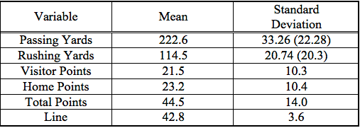
Table I contains some summary statistics for the data set. Teams averaged approximately 223 yards passing per game (offense or defense, of course) for the season, and they averaged approximately 115 yards rushing. The statistics reported on the rushing and passing standard deviations without parentheses are for the offenses and the defensive standard deviations are (as you might guess) in parentheses. Interestingly, passing defense is less variable across teams than is passing offense (we hypothesize that teams must be more balanced on defense to keep other teams from exploiting an obvious defensive weakness, but teams may be relatively unbalanced offensively and still be successful [see the 2011 Packers, for example, who ranked near the top in passing offense and near the bottom in rushing defense]). Home teams scored approximately 23.2 points on average for the season and outscored the visitors by 1.7 points. Total points averaged 44.5 in 2010-2011 and the over/under line averaged 42.8 (the difference between these means is statistically significant at α < .10; the calculated value for the t-test of paired samples is approximately 1.92). Not surprisingly, the standard deviation was much smaller for the line than for total points.
Table I: Summary Statistics
Regression Results
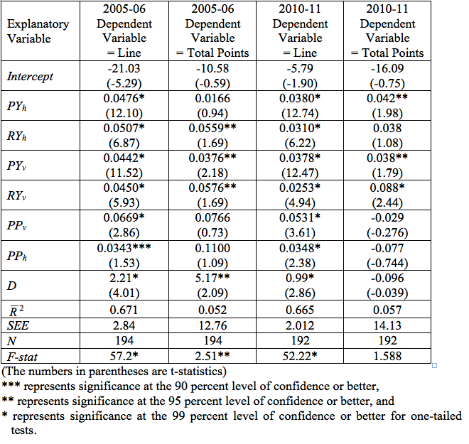
Though equations 1 and 2 from above represent our theoretical foundation, we did not find empirical support for the dome effect, points scored in the prior game, or for turnovers in predicting points for either the home or away teams. Thus we do not report regressions with those variables included (such estimations are available from the authors upon request). Since our objective is to produce predictions based on variables (and their effects) that are known prior to the games, we updated the equations weekly and checked for effects for those excluded variables. We did not find convincing evidence that any of the excluded variables should be included in the predictive equations.
The dome effect in a previous paper (see Pfitzner, Lang, & Rishel, 2009) found that teams scored approximately 5.4 more points when the game was played in a closed dome stadium for the 2005-2006 season. However, for the 2010-2011 season, games played in domes averaged 45.4 points and games played outdoors averaged 44.3. That difference is not statistically significant; the t-test for independent samples yields a calculated value of 0.54. The dome effect may be idiosyncratic in that, in some seasons, the high scoring teams may happen to be those who play home games in domed stadiums.
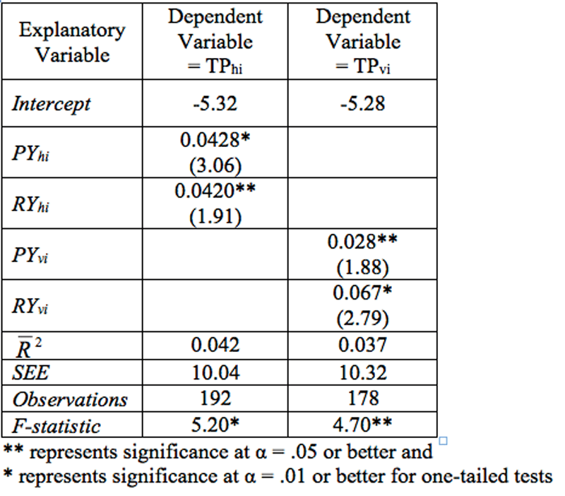
The representative estimated equations (at the end of the 16th week) are given in Table II. For the home points equation, the passing yardage and the rushing yardage are significant at α < .01, and α < .05 levels, respectively. The equation explains a modest 4.2% ( ) of the variance in home points scored. On the other hand, the F-statistic indicates that the overall equation meets the test of significance at α < .01. The estimated coefficients for the variables have the anticipated signs. To interpret those coefficients, an additional 100 yards passing (recall that this is the sum of the home team’s passing offense and the visitor’s passing defense) implies approximately 4.3 additional points for the home team, whereas an additional 100 yards rushing implies approximately 4.2 additional points.
Table II: Regression Results for Total Points Scored
The visiting team estimation yields a similar equation in terms of the overall fit. The explanatory variables are statistically significant—the passing yardage variable at α < .05, and the rushing yardage variable is significant at α < .01. The equation explains only 3.7% ( ) of the variance in visiting team points, and the F-statistic implies overall significance at α < .05. The coefficients perhaps suggest a more important role for rushing than for passing in scoring for the visiting team. If the coefficients are to be believed, an additional 100 yards passing yields approximately 2.8 points for the visiting team, and an additional 100 yards rushing is worth 6.7 points.
The reader may find such low values to be of concern, but recognize that the variables for which we are attempting estimates are very difficult to predict and are subject to wide variation. As we show in a later section, the lines on the games are much easier to predict. The model is best judged by its prediction qualities—here based on wagering success.
Other Hypotheses
Another hypothesis we wished to entertain is whether or not scoring is contagious. A priori, we surmised that points scored in given games for visiting and home teams would be positively related. In keeping with our earlier work, there is no evidence that such is the case. The estimated simple correlation coefficient between home team and visiting team points is -0.106, which is not statistically different from zero and “wrong” signed according to our intuition. Our initial thinking was that if team “A” scores and perhaps takes a lead, team “B” has greater incentive to score. An obvious complicating factor is that a given team may dominate time of possession, thus preventing the opposing team opportunities to score. We also experimented with two-stage least squares to test the hypotheses that scoring was contagious. In that formulation we developed a “predicted points” variable for the home team, entered that variable as an independent variable in the visiting team equation, and reversed the procedure for the home team equation. Neither of the predicted points variables were statistically significant. The variable was positively signed for the home team equation, and negatively signed for the away team equation.
As indicated above, we also find no evidence that teams are “streaky” with respect to points scored. In short, we find that points scored in the immediately prior week do not contribute to the explanation of points scored in the current week. That conclusion holds up for the regressions in section VI as well.
Finally, though turnovers clearly matter in who wins or loses, there is no evidence from our work that measuring teams’ turnovers per game prior to the current game aids in predicting points scored by the individual teams.
Wagering on the Over/Under Line
In this simulated wagering project we use the estimated equations to predict scores of the home and away teams for all of the games played over weeks 8 through week 17 (end of the regular season). The points predicted in this manner are then compared to the over/under line for each game. We then simulate betting strategies on those games.
Out-of-Sample Method
Since it is widely known that betting strategies that yield profitable results “in sample,” are often failures in “out-of-sample” simulations, we use a sequentially updating regression technique for each week of games. Suppose, for example, we are predicting points for week 8. We then estimate equations TPhi and TPvi with the data from weeks 5, 6, and 7, then “feed” those equations with the known data for each game through the end of week 7, generating predicted points for the visiting and home team for all individual games in week 8. The predicted points are then totaled and compared to the over/under line for each game. Next we add the data from week 8, re-estimate equations TPhi and TPvi, and make predictions for week 9. The same updating procedure is then used to generate predictions for weeks 10 through 17. This method ensures that our results are not tainted with in-sample bias.
Betting Strategies
We entertain three betting strategies for the predicted points versus the over/under line on the games. These strategies are:
1. Bet only games for which our predicted total points differ from the line by more than 7 points.
2. Bet only games for which our predicted total points differ from the line by more than 5 points.
3. Bet all games for which our predicted total points differ from the line by any amount—in our case, all games.
As stated previously, a betting strategy on such games must predict correctly at least 52.4% of the time to be successful. If a given method cannot beat this 52.4% criterion, as a betting strategy it is deemed to be a failure.
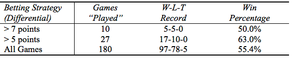
Table III contains a summary of the results for the three betting strategies. The first betting strategy yields only ten “plays” over weeks 6 to 17. That betting strategy would have produced five wins, and five losses. For this (very) small sample, this strategy is, of course, not profitable, with only a 50% winning percentage. The second strategy (a differential greater than 5 points) yields 39 plays and a record of 17-10-0—a winning percentage of 63%. Finally for every game played, the method produces a still profitable record of 97-78-5, with the winning percentage at 55.4%.
Table III: Results of Different Betting Strategies
There is some consistency between these results and those we found for the 2005-2006 season. In that work we found that the “> 5 points” strategy produced a winning percentage of 60.5% based on 39 plays. Betting all games produced a winning percentage of 54%. Interestingly, the earlier research produced nine games with a greater than 10 point difference between the line and the predicted points whereas this work on 2010-2011 season produced only one play (which would have been a winning bet).
It is important to note that we make no adjustment for injuries, weather, and the like that would be considered by those who make other than simulated wagers. We offer these methods only as a guide, not as a final strategy.
Another Method of Predicting the Line and Total Points
Since we have collected and created variables that may be relevant to determining the betting line (and total points), in this section we investigate the relevancy of our variables in that context. For purposes of comparison, we estimate an equation for the over/under line and, separately, for the actual points scored. Further, we compare the results for the 2010-11 season with our results from prior research. These equations may be useful in confirming (or contradicting) the results of the previous sections, and may provide useful information applicable to wagering strategies.
The results of those regressions are contained in Table IV. We estimated regression equations for two seasons with the line as the dependent variable and all of the right-hand side variables (with the exception of turnovers) specified in equations 1 and 2. The estimations for the line are contained in the second column (2005-2006 season) and the fourth column (2010-2011 season). The estimations are remarkably similar. For the line for both seasons, every coefficient estimate is correctly signed and statistically significant at traditional levels of alpha, and for both equations. The line seems to be set on the assumption that teams are streaky (we conclude they are not), and the dome effect on the betting line seems to be a bit smaller in the most recent season.
Table IV: Regression Results for the Line and Total Points, 2005 and 2010 Seasons
As a comparison, we also estimated (far less successfully) an equation for total points with the same set of explanatory variables with those results reported in columns three and five of Table IV. Perhaps the most striking result of these regressions is that the regressions for the line explain fully two-thirds of the variance in that dependent variable and the equations for the actual points explains less than 6% of the variance in total points for either season, with only four of the seven explanatory variables meeting the test for statistical significance at traditional levels for 2005-2006 and only three for 2010-2011. Interestingly, the dome effect for total points for the earlier season estimated 5 additional points scored in dome games, and the corresponding estimate for the 2010-11 season was zero, when controlling for other effects. Recall that for the 2005-2006 season, 5.4 points more were scored in games played in domes, and the corresponding difference was only one point for the 2010-2011 season.
In short, and to be expected, the line is much easier to predict than is actual points scored. That is, the outcome of the games and points scored therein are not easily predicted. It is tempting to say, “That’s why they play the games.” At least two further observations are in order. First, consider the coefficients for points scored in the previous game. Those variables matter as would be anticipated on an a priori basis in determining the line for the game. However, they seem to play an insignificant (statistical or practical) role determining the actual points scored. This particular result may be interpreted as bettors placing too much emphasis on recent information, as other authors have suggested.
Finally, it also seems clear that the effect of playing indoors has dissipated between the two seasons for which we report results in Table IV. As we have emphasized, this may be simply the effect of teams who play many games indoors having poorer scoring teams for any particular year.
CONCLUSIONS
The regression results in this paper identify promising estimating equations for points scored by the home and away teams in individual games based on information known prior to the games. In a regression framework, we apply the model to three simulated betting procedures for NFL games during weeks 6 through 17 of the 2010-2011 season. Betting strategies based on the differences between our predictions and the over/under line produced profitable results for either all games at any differential or those for which our predictions differed from the betting line by 5 or more points.
Based on our earlier results finding profitable wagering strategies for the 2005-2006 season, we (and others) questioned whether these results will hold up in other seasons. Based on the results presented here—so far, so good.
APPLICATIONS IN SPORT
Betting on sports, the NFL in particular, is a very popular pastime among sports (or gambling) enthusiasts and a very lucrative business for bookmakers in Las Vegas and elsewhere. This research was conducted to determine whether successful wagering strategies could be developed based on regression equations used to predict points for the home and away teams in individual games. The sum of the predictions for the home and away teams, updated weekly, were then compared to the over/under line on individual NFL games. Certain betting strategies were identified as successful, and could therefore be used by those wanting to improve their odds while enjoying and increasing their interest in America’s favorite sport.
ACKNOWLEDGMENTS
None
REFERENCES
1. Badarinathi, R., & Kochman, L. (2001). Football betting and the efficient market hypothesis. The American Economist, 40(2), 52-55.
2. Borghesi, R. (2007). The home team weather advantage and biases in the NFL betting market. Journal of Economics and Business, 59, 340-354.
3. Boulier, B. L., Steckler, H. O., & Amundson, S. (2006). Testing the efficiency of the National Football League betting market. Applied Economics, 38, 279-284.
4. Dare, W. H., & Holland, A. S. (2004). Efficiency in the NFL betting market: modifying and consolidating research methods. Applied Economics, 36, 9-15.
5. Dare, W. H., & MacDonald, S. S. (1996). A generalized model for testing home and favourite team advantage in point spread markets. Journal of Financial Economics, 40, 295-318.
6. Gray, P. K., & Gray, S. F. (1997). Testing market efficiency: Evidence from the NFL sports betting market. The Journal of Finance, LII(4), 1725-1737.
7. Levitt, S. D. (2002). How do markets function? An empirical analysis of gambling on the National Football League. National Bureau of Economic Research (Working Paper No. 9422).
8. Paul, R. J., & Weinbach, A. P. (2002). Market efficiency and a profitable betting rule: Evidence from totals on professional football. Journal of Sports Economics, 3, 256-263.
9. Pfitzner, C. B., Lang, S. D., & Rishel, T. D. (2009). The determinants of scoring in NFL games and beating the over/under ;ine. New York Economic Review, 40, 28-39.
10. Pfitzner, C. B., Lang, S. D., & Rishel, T. D. (2006). Can regression help to predict total points scored in NFL games? In A. Avery (Ed.), The 2006 Southeastern INFORMS Conference Proceedings (pp. 312-317). Myrtle Beach, SC: Southeastern INFORMS.
11. Vergin, R. C. (2001). Overreaction in the NFL point spread market. Applied Financial Economics, 11, 497-509.
Submitted by Anja Pečaver, Maja Pungeršek, Mateja Videmšek, Damir Karpljuk, Jože Štihec and Maja Meško.
ABSTRACT Purpose: The study deals with an analysis of teaching swimming to children aged between four and eleven.
Methods: The study involved swimming instructors, teachers and coaches from different swimming schools in Slovenia. Data were acquired for 90 providers of swimming courses. The data were then analysed using descriptive statistic methods. The hypotheses were verified using Pearson’s χ² test and the Mann-Whitney test. Statistical significance was established at a 5% risk level.
Results: It was established that the differences between some parts of the exercise unit in terms of the frequency of use of a didactic movement game were related to gender and the acquired professional title. The didactic tools most frequently used during the swimming classes include kickboards, floating noodles and pool dive toys.
Conslusion: Children become more enthusiastic about learning to swim if information communication technology and didactic devices are used; it is easier to motivate them and attract their attention.
Applications in Sports: Swimming teachers should more often use didactic flotation devices whitch will fullfil children’s interest for swimming.
INTRODUCTION
It is extremely important for children to engage in a sport activity. Already at an early age they should be offered a variety of motor activities so as to broaden their horizons (16). In recent times, the age limit at which a child is expected to swim and have good swimming knowledge has decreased considerably. These days we expect children to swim already at the start of primary school whereas in the past children developed this ability at the end of primary school (17). Many reasons speak in favour of teaching children to swim as early as possible, with one of them clearly being to protect them from drowning. This is one reason that the new physical education curriculum for primary schools (10) includes a compulsory 20-hour swimming course in the second or third grade (at the age of 7–9 years). According to British experts, the most appropriate time to learn to swim is the three-year period from the age of eight to eleven because the learning process is fast and relaxed, children are motivated and few pupils skip classes (6). Relying on the results of her study, Škafar Novak (18) states it is reasonable to teach swimming at two age levels, namely getting children accustomed to water in the first primary school grade (6–7 years) and teaching them to swim in the third primary school grade (8–9 years). Great progress in swimming “literacy” is seen already with the youngest generations who explore water and its environment. Today about 10% of babies at the age of six months and older (17) can swim. Moreover, an analysis of reports on the running of annual sport programmes in local communities reveals that 249 swimming courses were conducted in 2008 (186 in primary schools, 63 in kindergartens) involving a total of 8,972 children (9).
When learning to swim it is important that the programme underpinning the learning process is well structured and suitable for the specific age group and the previous knowledge of the learners, and that it is organised flawlessly (4, 14). Incorrect steps taken during a child’s first contact with water can considerably extend the process of learning to swim and result in a negative experience which could linger throughout their life (12, 19). We should be aware that children’s safety is crucial in all types of sport activities, and just as important as maintaining their positive attitude to sport. All of the above depend more or less on the teacher who must be acquainted with the various contents, methods and types of learning to be able to attain the set goals. Working with young age groups is particularly demanding as it requires special approaches, gradual work and reasonable planning of the entire training process.
When one thinks about water activities for children, images of joy, fun, pleasure and laughter come to mind. To maintain such positive feelings during exercise and also afterwards, the swimming instructor/teacher/coach must not only have good knowledge of swimming techniques and good demonstration skills but also master appropriate swimming teaching methods which, for young children, must be based on didactic play. Jurak and Kovač (6) emphasise that the number of lessons making up the swimming “literacy” campaign has been decreasing which is why the teacher must make the best of the time that is dedicated to learning swimming. This can be achieved by using a modern learning programme which also includes the use of an appropriate didactic movement game and a variety of didactic tools (12, 25).
Given the obstacles that commonly appear on the way to the set goal, swimming professionals must cope with different situations, some of which may be very stressful for both the learners and teachers alike. It is up to the teacher which method they will choose to solve the problems, and their choice depends on their education, work experience and mainly their gift for working with children. Kovač (10) established that children up to nine years of age are most often taught by professionals with the title “swimming instructor” who generally have 3 to 5 years of work experience. They use a variety of didactic tools in their work which is positively reflected in the high motivation of children and, consequently, the high percentage of children who have become completely accustomed to water by the end of the course.
The purpose of the study was to analyse the teaching of swimming to children aged between four and eleven. We aimed to establish which difficulties swimming instructors/teachers/coaches encounter in individual exercise units, to what extent they use different didactic tools and a didactic movement game. Another aim was to establish whether there were any statistically significant gender differences in terms of the selection of the group of learners, the frequency of use of a didactic movement game and the frequency of coping with problems related to the learner’s personality. Another aim was to establish any statistically significant differences in the frequency of use of a didactic movement game depending on the professional title acquired by the instructor/teacher/coach.
WORK METHODS
Study subjects
The study encompassed a sample of 90 professionals (71 swimming instructors, 16 swimming teachers and 3 swimming coaches) who conduct swimming courses in different places in Slovenia. The sample of subjects included 57.8% of women aged between 20 and 50 and 42.2% of men aged between 19 and 55 years. The survey questionnaires were handed out during a licensing seminar for swimming instructors.
Swimming aids
The study was underpinned by a survey questionnaire which was completed by instructors, teachers and coaches from different swimming schools in Slovenia. The survey questionnaire included 15 questions of which some were closed-ended while others involved a combination of open-ended and closed-ended questions. Absolute anonymity of the subjects was ensured.
Verification of the questionnaire’s reliability
Cronbach’s alpha is a coefficient of reliability or consistency. Its purpose is to establish how effectively a group of variables or items measures an individual one-dimensional latent composition. With a multidimensional structure the alpha coefficient is low (13).
The value of Cronbach’s alpha rises with an increase in the number of items in the questionnaire. When correlations between the items are low, the value of alpha is also low: the higher the correlation, the higher the alpha value. High correlations among the items prove that the latter are measuring the same basic problem or subject. In that case, we can conclude that their reliability is good, i.e. high. It has been assessed in theory that alpha values around 0.60 are still acceptable (13).
It was concluded that the questionnaire’s reliability is high ranging from 0.72 to a very high value of 0.816.
Procedure
The 90 swimming instructors, teachers and coaches who attended the licensing seminar for swimming instructors at the Faculty of Sport in Ljubljana received the survey questionnaires. The data were processed with the SPSS 19.0 (Statistical Package for the Social Sciences) software application. The Mann-Whitney test and Hi² test were conducted. Statistical significance was established at a 5% risk level.
Limitations of the study
The study was conducted among swimming teachers in Slovenian primary schools. The study is thus limited to Slovenia in geographical terms. It does not encompass any teachers of children with special needs and does not investigate the characteristics and problems of the didactical teaching of children with special needs.
RESULTS
The results of the survey questionnaire served as a basis for analysing the system of work in different swimming schools in Slovenia.
The analysis of work experience revealed that professionals with 3 to 4 years of experience (31.1%) were in the majority, followed by those with 1 to 2 years (26.6%) and those with 5 to 6 years (23.3%) of experience. The smallest share was that of professionals with 7 years of experience or more (18.9%).
More than three-quarters of the surveyed professionals attend expert seminars once every two years to refresh their previous knowledge and acquire new knowledge. This result was expected since most of the surveyed professionals hold the swimming instructor licence which must be ratified every two years by attending expert seminars. Ten percent of the subjects attend seminars once a year and 3.3% twice a year. Surprisingly, 11.1% of those surveyed answered that they never attend any seminars.
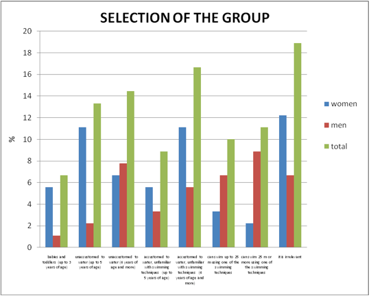
We were also interested in which children they would prefer to select for their group (Figure 1) and whether there were any statistically significant differences in terms of the professionals’ genders (Table 1).
Figure 1. Selection of a group depending on a professional’s gender
Only 18.9% of the surveyed professionals answered that it was irrelevant which group they teach, whereas others chose a group based on the learners’ age and knowledge. The results show that women prefer to teach the youngest children who are not yet accustomed to water or are unfamiliar with the swimming techniques, whereas men prefer learners who are accustomed to water and can swim 25 metres or more using one of the swimming techniques (Figure 1).
Table 1. Selection of a group depending on a professional’s gender
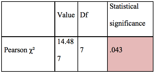
It can be asserted at a 5% risk level that there are statistically significant differences in the selection of a group in terms of the gender of the swimming instructor/teacher/coach (Table 1).
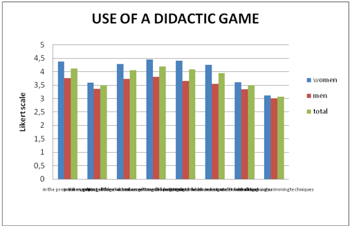
Given the importance of playing for the overall development of a child, the surveyed professionals were asked how frequently they used didactic movement games when teaching children to swim (Figure 2).
Figure 2. Use of a didactic game in the teaching of swimming
Using a 5-point Likert scale (with 1 meaning never and 5 always) the surveyed professionals assessed that they use a didactic movement game most often when getting children accustomed to putting their head under water (4.19), followed by the preparatory part of the exercise unit (4.12) and getting children accustomed to seeing under water (4.09). These are followed by getting children accustomed to exhaling in water (3.96), while sliding and in the main part of the exercise (both 3.5). The professionals use a didactic movement game the least in the actual teaching of swimming techniques (3.07) (Figure 2).
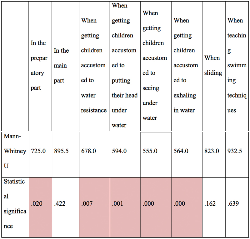
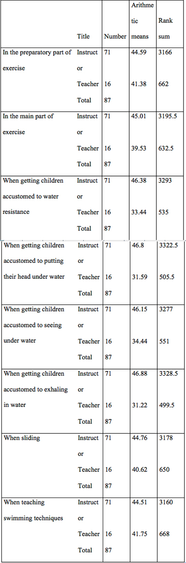
We were interested in whether any statistically significant differences in the frequency of using a didactic movement game when teaching swimming depend on a professional’s gender (Table 2).
Table 2. Use of a didactic motor game in specific parts of the exercise unit, with different contents, depending on a professional’s gender
It can be asserted at a 5% risk level that there are statistically significant differences in the frequency of use of a didactic movement game in the preparatory part of the exercise unit, when getting children accustomed to water resistance, putting their head under water, seeing under water and exhaling in water (Table 2). The female professionals use didactic movement games more frequently when teaching the abovementioned activities (Figure 2).
We were interested in whether any statistically significant differences in the frequency of use of a didactic movement game in the teaching of swimming depend on a teacher’s gender (Table 3).
Table 3. Use of a didactic movement game in the exercise unit depending on the acquired professional title
It can be asserted at a 5% risk level that there are statistically significant differences in getting children accustomed to water resistance, putting their head under water and exhaling in water (Table 3). The swimming professionals with lower titles (swimming instructors) more frequently use a didactic movement game in the abovementioned activities than the professionals who hold higher titles (swimming teachers).
Table 4. Use of a didactic movement game in specific parts of the exercise unit depending on the professional title
The frequency of the use of different didactic tools during the teaching process was also analysed (Figure 3).
Figure 3. Use of swimming aids
Analysis of the results shows (Figure 3) that in swimming schools the three most frequently used didactic tools include a kickboard (4.24), a floating noodle (4.11) and pool dive toys (3.60). Of all the above mentioned swimming aids the professionals only occasionally use pull buoys, swim hats/floating toys and rings/frames and only rarely mats and slides, whereas swimming balls and swimming belts are almost never used.
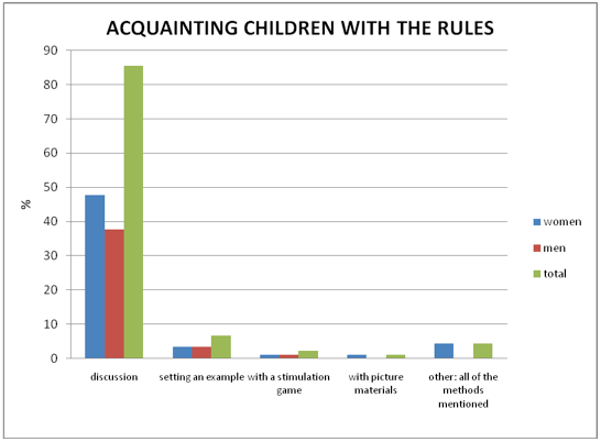
We were interested in how the swimming instructors/teachers/coaches acquaint children with the rules that must be observed in the swimming pool (Figure 4).
Figure 4. The method of acquainting children with the rules
The professionals most often employ the discussion method (85.6%). Less than 14% of the answers to this question fit into the categories: by setting an example, using a stimulation game, with picture materials and by using all of the methods mentioned (Figure 4).
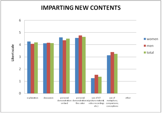
The respondents were asked how they impart new swimming contents to children. They had to mark the listed learning methods from 1 to 5, with 1 meaning never and 5 always (Figure 5).
Figure 5. Method of imparting new contents
Figure 5 shows that a personal demonstration in the water is the method professionals use in almost every exercise unit to impart new contents to children (4.64). Personal demonstration on land ranks second (4.5). The professionals often use the explanation and discussion methods (4.19 and 4.13, respectively). Sometimes they use metaphors, comparisons (e.g. leap like a dolphin) and conceptions (3.24). It is surprising that they almost never use picture materials and video recordings (1.37).
In the study, we enquired into the problems the instructors/teachers/coaches deal with during the pedagogical process (Figure 6).
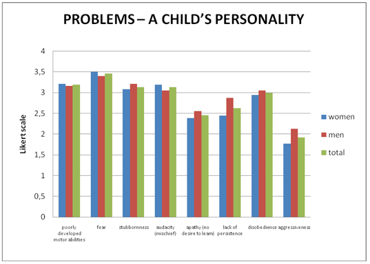
Figure 6. The frequency of problems related to a child’s personality the professionals deal with
Figure 6 shows that the professionals most frequently deal with fear (3.46) during swimming lessons. In terms of the frequency of occurrence, that is followed by motor abilities (3.19), stubbornness and audacity or mischief (3.13). Disobedience (2.99) is also in the middle of the range. The sixth place in terms of frequency is held by lack of persistence (2.62) and the penultimate one to apathy (2.46). The least frequent is aggressiveness (1.93).
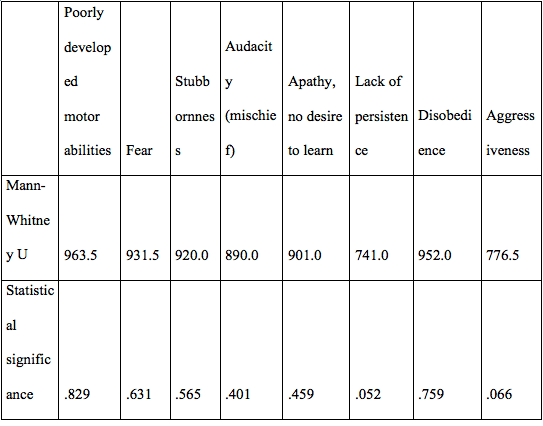
We were also interested in whether any statistically significant differences in the frequency of dealing with problems related to a child’s personality depend on a professional’s gender (Table 5).
Table 5. Frequency of dealing with problems depending on a professional’s gender
It can be asserted at a 5% risk level that there are no statistically significant differences in the frequency of dealing with problems related to a child’s personality that depend on a professional’s gender (Table 5).
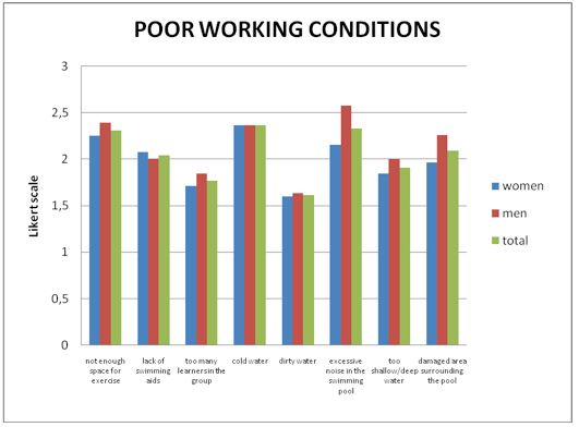
A prerequisite for the high-quality implementation of swimming courses is a swimming facility which complies with basic health, safety and pedagogical standards. The surveyed professionals were asked how frequently they encounter poor working conditions (Figure 7).
Figure 7. Frequency of encountering poor working conditions
Figure 7 shows that the surveyed professionals most often deal with cold water – it was graded with 2.37 points, which means they encounter it sometimes. The next two are excessive noise in the swimming pool (2.33) and not enough space for exercise (2.31). Only rarely do the professionals deal with a damaged area surrounding the pool (2.09), a lack of swimming aids (2.04), too shallow/deep water (1.91), too many learners in the group (1.77) and the last-ranking dirty water (1.61).
At the end the swimming instructors/teachers/coaches were asked to explain how they choose the method for resolving problems encountered during the pedagogical process (Figure 8).
Figure 8. Demonstration of the frequency of problem-solving methods
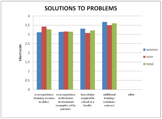
The surveyed professionals most often choose the problem solving methods they became acquainted with during additional trainings such as seminars and courses; these methods were assessed with 3.60. Slightly fewer professionals use methods stemming from their own experience acquired during training sessions in clubs or sport societies (3.27). In third place is knowledge acquired in school and/or at a faculty (3.21). Professionals help themselves the least with the experience they have acquired in their home environment based on behavioural patterns in the family and the examples set by parents. This was assessed with 3.14.
DISCUSSION
Teaching young children to swim requires the use of methodical procedures, good knowledge of different games and the handling of swimming aids as well as a lot of patience, dedication and energy (14). The study established that women prefer to teach the youngest children, especially those who are not yet accustomed to water or are unfamiliar with the swimming techniques, whereas men prefer to teach children who are already accustomed to water and can swim 25 metres or more using one of the swimming techniques.
Emotional learning takes place as long as there is an emotional link with the subject of learning; when the link is broken, children become weary and they turn their attention to other things and no longer accept information. If the games are carefully chosen they will engage the child’s emotions sufficiently (2, 11, 21). The study shows that swimming professionals only occasionally use a didactic movement game in the actual teaching of swimming techniques. This is of great concern because it shows that swimming professionals are not aware that children, even when they are already accustomed to water, are still children whose basic desire, need and right is to play and to enjoy playing. The results show that professionals with lower titles (swimming instructors) and who are female use didactic games in some swimming course activities considerably more than men. Playfulness is the prerequisite for a game and should combine freedom, relaxedness and an absence of fear. We believe that too many instructors/teachers/coaches refuse to rediscover the child within themselves and to descend to the child’s level, or are incapable of doing this. In their analysis of skiing teaching methods for the youngest, Dobida and Videmšek (5) also established that didactic games were much too rarely used in practice and that their use declines with the increasing skiing knowledge of a child.
The use of appropriate didactic tools adds to the quality of the exercise, while also making it more lively (8). The analysis of the results shows that in swimming schools the three most frequently used didactic tools included kickboards, floating noodles and pool dive toys. In fact, these are very commonly used swimming aids and can be used to get a learner accustomed to water and to teach them the basics of the swimming technique. Of all the above mentioned aids, swimming professionals occasionally use pull buoys, swimming hats/floating toys and rings/frames and only rarely mats and slides, whereas swimming balls and swimming belts are almost never used. The abovementioned aids break the monotony of the exercise, enable the learner to gain some independence in the water and provide for diversity in the learning process, and so they are an important motivational tool for learners. It is important that the aids are suitable (made of safe materials), in vivid colours, of the appropriate size etc. (22). Sometimes, the use of didactic tools for teaching non-swimmers was limited solely to a kickboard and balls or, in many cases, there were no tools at all (6, 15). Today, swimming instructors/teachers/coaches have many didactic tools available that enable the transfer of information in the psychomotor cognitive process; they facilitate the demonstration of a specific movement as well as the transfer and acceptance of different pieces of information which influence the final knowledge of the swimming course participant. It is difficult to imagine any sport activity without appropriate tools. An exercise becomes dull and is difficult to implement, especially with the youngest children. Didactic tools should be selected based on the set goals and children’s level of development. The availability of tools most often depends on financial resources; however, with a little resourcefulness one can make tools by themselves or borrow them.
In all sport exercises specific rules and regulations apply that must be followed by those implementing activities and the learners. Also in a pool or a swimming facility one must observe the rules and, most importantly, respect oneself and other people. The purpose of the signs set up around pools and swimming facilities is to inform swimmers about the water depth, prohibitions and types of danger (14). Therefore, we were interested in studying how the swimming instructors/teachers/coaches acquaint children with the rules that must be observed in the swimming pool. The swimming professionals most often only employ the discussion method. Only a few professionals set their own example, use a stimulation game and picture materials even though these are the methods that attract a child’s attention the most.
The surveyed professionals were asked how they impart new swimming contents to children. The demonstration method plays a particularly important role in the implementation of a physical education process for the youngest. It allows children to obtain a clear idea of the movement they are expected to perform. The analysis of the answers to the abovementioned survey questions shows that the professionals are aware of the above, as personal demonstration in the water and personal demonstration on land were ranked first and second, respectively. The professionals often use the explanation and discussion methods. Learning strategies are quite rarely used, namely, comparisons, metaphors and conceptions functioning as cognitive aids in the process of learning new contents and systematically supporting cognitive processes related to knowledge and the acquiring of new knowledge (1, 23). Those who run swimming courses know too little about the learning strategies which help learners achieve the set goals faster and easier. The swimming professionals almost never use picture material and video recordings. Children become more enthusiastic about learning to swim if information communication technology is used; it is easier to motivate them and attract their attention.
As a group consists of children with different behavioural characteristics and peculiarities, many things can happen while teaching them to swim (11). We enquired about the problems instructors/teachers/coaches deal with during the pedagogical process. The surveyed professionals noted that the greatest burden is a child’s fear of water which is a consequence of their negative experience with water. This fear is often unintentionally created by parents and the heads of swimming courses if they incessantly warn children about the dangers of water. As expected, the second place was occupied by poorly developed motor abilities of children which represent a great problem of modern times. Namely, children spend most of their leisure time at home, watching TV or sitting in front of a computer. Fear and poor motor abilities are followed by stubbornness, audacity and disobedience. We established no statistically significant differences in the frequency of dealing with problems related to the child’s personality depending on a swimming professional’s gender. All of the abovementioned problems are a consequence of the fast pace of living since these days parents do not spend enough time with their children. The latter learn many things from TV shows and computer games. The last three places among all problems were taken by a lack of persistence, apathy and aggressiveness. In one of their studies, Štihec, Bežek, Videmšek, and Karpljuk (20) found that physical education teachers often have to cope with a lack of discipline, excessive boisterousness, a failure to follow instructions, unauthorised absences, pupils’ lack of motivation, potentially dangerous situations/activities for pupils etc. during their work which can lead to a conflict situation.
The prerequisite for the high-quality implementation of a swimming course is appropriate working conditions. The swimming facility must meet basic health, safety and pedagogical standards (3). The surveyed professionals were asked how frequently they encounter poor working conditions and they ranked contact with cold water at the top of the problem list. Therefore, it is very important that children do not stand still during the swimming course but perform different motor tasks all the time. The surveyed professionals also reported that excessive noise in the swimming pool and insufficient space for exercise were quite annoying. Only rarely do the professionals deal with a damaged area surrounding the pool, a lack of swimming aids, too shallow/deep water, too many learners in the group and dirty water.
If the swimming instructors/teachers/coaches encounter problems during the pedagogical process they most often choose problem-solving methods they have learned about during additional trainings such as seminars and courses. In second place is the method stemming from their own experience which was acquired during trainings in clubs or sport societies. This is followed by knowledge acquired at school or a faculty, whereas the method the instructors/teachers/coaches use the least is their experience they have acquired in their home environment (examples set by parents and other members of the family).
CONCLUSION
The swimming learning model has been developed in Slovenia for already 50 years. The Slovenian theoretical design and practical implementation have thus approached the models of some of the most developed European countries such as Sweden and the Netherlands (7). In slightly less than a decade, swimming knowledge in Slovenia has improved by almost 20% due to the systematic approach to individual levels of the teaching of swimming, monitoring of an individual’s progress after each level, the intertwining of compulsory and elective school programmes as well as the projects within the National Sport Programme, a number of systemic measures throughout all these years and public co-financing (9).
The quality of the teacher’s expert work primarily depends on their professional qualifications or knowledge, personality, abilities, creativity and authority (8, 24). When teaching the youngest, one should be aware that children are not just a miniature copy of adults but are specific learners with their own needs, requirements and last but not least desires. One has to be familiar with the different paths to the goal that must be adjusted to children. Therefore, when teaching these age categories swimming instructors/teachers/coaches must consider a child’s developmental characteristics, adjust the didactic approaches and include different didactic tools in the process. Finally, it is very important that learning to swim becomes a pleasant and interesting experience for the child, that it awakens positive feelings in them so that they will continue to engage in recreational swimming later in life.
APPLICATIONS IN SPORT
We have to be aware that a didactic game is a fundamental method of work and approach to working with children, but the study shows that swimming professionals only occasionally use a didactic movement game in the actual teaching of swimming techniques. Therefore didactic motor game is still underused in practice; its use decreasing with the increasing level of child’s swimming skills. Children need and right is to play and to enjoy playing, so swimming teachers should more often use didactic flotation devices.
ACKNOWLEDGMENTS
Authors agree that this research has non-financial conflicts or interest. This includes all monetary reimbursement, salary, stocks or shares in any company.
REFERENCES
1. Anderson, A. T. (2002). Manjkajoča misel: strategije poučevanja v športni vzgoji in vrhunskem športu [The missing thought: Teaching strategies in physical education and elite sport]. Ljubljana: Sport Teachers Association: Slovenian Sports Institute: Faculty of Sport.
2. Coakley, J. (2011). Youth sports what counts as “positive development”. Journal of Sport & Social Issues, 35(3), 306–324.
3. Coates, E., & Coates, A. (2007). Young children talking and drawing. International Journal of Early Years Education, 14(3), 221–241.
4. Dybinska, E., & Kaca, M. (2007). Self-assessment as a criterion of efficiency in learning and teaching swimming. Human Movement, 8(1), 39–45.
5. Dobida, M., & Videmšek, M. (2005). Analiza poučevanja alpskega smučanja najmlajših [Analysis of teaching of Alpine skiing to the youngest]. Šport, 53(4), 49–53.
6. Jurak, G., & Kovač, M. (2002). Izbor didaktičnih pripomočkov za učenje plavanja [Selection of didactic tools for teaching swimming]. Ljubljana: Ministry of Education and Sport, Sport Department.
7. Jurak, G., & Kovač, M. (2010). Izpeljava športne vzgoje: didaktični pojavi, športni programi in učno okolje [Implementation of physical education: Didactic phenomena, sport programmes and learning environment]. Ljubljana: Faculty of Sport, Centre for Lifelong Learning in Sport.
8. Kapus, V., Štrumbelj, B., Kapus, J., Jurak, G., Šajber, D., Vute, R., Bednarik, J., Šink, I., Kapus, M., & Čermak, V. (2002). Plavanje, učenje [Swimming, learning]. Ljubljana: Institute of Sport, Faculty of Sport, University of Ljubljana.
9. Kolar, E., Jurak, G., & Kovač, M. (2010). Analiza nacionalnega športa v Republiki Sloveniji 2000–2010 [Analysis of national sport in the Republic of Slovenia 2000–2010]. Ljubljana: Sports Federation for Children and Adolescents of Slovenia.
10. Kovač, K. (2011). Analiza tečajev plavanja mlajših otrok [Analysis of swimming courses for young children]. Graduation thesis, Ljubljana: University of Ljubljana, Faculty of Sport.
11. Light, L.R. (2010). Children’s social and personal development through sport: A case study of an Australian swimming club Sport & Social Issues, 34(4), 379–395.
12. Light, R., & Wallian, N. (2008). A Constructivist-Informed Approach to Teaching Swimming. Quest, 60(3), 387–404.
13. Nunnally, J. C., & Bernstein, I. H. (1994). Psychometric theory (3rd ed.). New York: McGraw-Hill.
14. Pečaver, A. (2011). Analiza poučevanja plavanja mlajših otrok [Analysis of teaching young children to swim]. Graduation thesis, Ljubljana: Faculty of Sport.
15. Rajtmajer, D. (1994). Metodično-didaktični problemi edukacije otrok z vidika (ne)uporabe didaktičnih medijev [Methodical-didactical problems in children’s education in terms of the (non)use of didactic tools]. In Proceedings of the 1st Slovenian Consultation on Teaching of Swimming and Safety from Drowning (pp. 213–217). Ljubljana: Faculty of Sport, Institute of Sport.
16. Swanson, J., Raab, M., & Dunst, J.C. (2011). Strengthening family capacity to provide young children everyday natural learning opportunities. Journal of Early Childhood Research. 9(1), 66–80.
17. Šajber, D. (2006). Plavanje od rojstva do šole [Swimming from birth to school]. Radovljica: Didaktika.
18. Škafar Novak, U. (2007). Primerjava učinkovitosti učenja plavanja med 6-7- in 8-9-letniki [A comparison of swimming learning efficiency between 6–7 and 8–9 year old children]. Graduation thesis, Ljubljana: University of Ljubljana, Faculty of Sport.
19. Štemberger, V. (2005). Plavanje v prvem triletju devetletne osnovne šole [Swimming in the first triad of the nine-year primary school]. In Proceedings / 2nd Expert Consultation on Didactics in school and nature (pp. 166–170). Ljubljana: Center šolskih in obšolskih dejavnosti.
20. Štihec, J., Bežek, M., Videmšek, M., & Karpljuk, D. (2004). An analysis of how to solve conflicts of physical education classes. Gymnica, 34(1), 23–29.
21. Videmšek, M., & Pišot, R. (2007). Šport za najmlajše [Sport for the youngest]. Ljubljana: Faculty of Sport, Institute of Sport.
22. Videmšek, M., Štihec, J., & Karpljuk, D. (2008). Analysis of preschool physical education. Ljubljana: Faculty of Sport, Institute of Kinesiology.
23. Wallis, J., & Binney, J. (2010). Learning and teaching through swimming and water-based activities. In, The really useful physical education book: learning and teaching across the 7–14 age range. Stidder, G (Ed.). Taylor & Francis; pp. 104–118.
24. Wiesner, W. (2008). Swimming education – the area of interest and methodological basis. In Science in Swimming, Zatona, K, Jaszczak, M (Eds). Wroclaw; Wydawnictwo AWF; pp, 41–48.
25. Woodson, E. D., Timm, F. D., & Jones, D. (2011). Teaching kids about healthy lifestyles through stories and games: Partnering with public libraries to reach local children. Journal of Hospital Librarianship, 11(1), 59–69.
Submitted by Christie Zunker, PhD, Trisha Karr, PhD, Roberta Trattner Sherman, PhD, FAED, Ron A. Thompson, PhD, FAED, Li Cao, MS, Ross D. Crosby, PhD and James E. Mitchell, MD.
ABSTRACT
This study examined the relationship between clothing fit and perceived fitness level. Participants included 2,386 adults who completed an online survey after a running event. The survey included four questions related to photographs of athletic models wearing loose-fitting and tight-fitting clothing: (1) Which event do you think the model took part in? (2) What do you think is the main reason he/she took part in the event? (3) How well do you think this person performed? and (4) How confident are you that your running time beat this person’s time? Results showed participants were more likely to believe athletes wearing tight-fitting clothing ran further and faster than athletes wearing loose-fitting clothing; and were less confident in their abilities to run faster than athletes wearing tight-fitting clothing than those who wore loose-fitting clothing.
These findings suggest clothing fit influences perception of athletic ability among runners. Athletes making upward comparisons may become increasingly dissatisfied with their appearance and at risk for avoidance of certain sports, decreased amounts of time spent in moderate to vigorous physical activity, and experience feelings of inferiority that negatively influence sport performance.
INTRODUCTION
Sociocultural comparisons and perceived pressure to be thin can foster body dissatisfaction (15); however, some individuals report a preference for athletic-ideal body shapes over a thin-ideal (13). Comparing oneself to a fit peer can affect body satisfaction and the amount of time one engages in physical activity. For example, a study by Wasilenko and colleagues (2007) with female undergraduates found that women stopped exercising sooner and felt less satisfied with their bodies when they exercised near a woman they perceived as physically fit wearing shorts and a tight tank top as compared to exercising near an unfit woman wearing baggy pants and a baggy sweatshirt (23). Thus, social comparisons with peers may promote unhealthy behaviors or avoidance of certain activities. Additionally, individuals who experience weight-related stigmas may be less willing to participate in physical activity and avoid exercise due to low perceived competence and lack of motivation (16, 22).
Individuals who adopt an external observational view, or a self-objectified perspective of their bodies, may invest a considerable amount of psychological, physical, and financial resources into their appearance (1). Objectification theory proposes that these individuals internalize the observers’ view of their bodies (i.e., self-objectification) and become preoccupied with how their body appears to others without regard to how their body actually feels (10). Interviews with elite athletes indicate that they view an athlete’s body “as an object to be managed” (17p. 206). Self-objectifying thoughts and appearance concerns may be triggered in individuals with low self-esteem and exacerbated in certain environments (e.g., gyms with mirrors, women wearing revealing outfits;18). For example, a study by Fredrickson and colleagues (1998) in which participants (70% Caucasian) were instructed to try on either a swimsuit or a sweater in a dressing room with a full-length mirror and then complete a mathematics test showed that women in the swimsuit condition performed worse on the test than women in the sweater condition. The authors postulated that bodily shame diminished their mathematical performance since their mental energy was focused on their appearance (11). Another study by Hebl and colleagues (2004) with a similar protocol with men and women of Caucasian, African American, Hispanic, and Asian American descent, found that all participants had lower mathematics performance and appeared vulnerable to self-objectification during the swimsuit condition compared to the sweater condition (12). A study by Fredrickson and Harrison (2005) with 202 adolescent girls found that those with higher measures of self-objectification had poorer performance throwing a softball when asked to throw as hard as she could (9). These findings suggest that experiencing bodily shame may negatively influence one’s ability to engage in physical activities or other activities that require mental resources.
Clothing appears to be an important, but often ignored, part of how women manage their physical appearance (21). Wearing a swimsuit or other tight, body contouring uniform for a particular sport may be necessary for performance, but there are often gender discrepancies with women usually wearing much less clothing (19). Revealing sports uniforms may be perceived as stressors and exert pressure on some athletes functionality or performance advantage. Indeed, some individuals report feeling uncomfortable wearing revealing attire and may choose not to participate in a particular sport due to required uniforms.
Sports uniforms may contribute to unhealthy eating behaviors and eating disorders, especially among women. For example, female athletes often experience increased body image concerns, unhealthy body comparisons, and body dissatisfaction; however, satisfaction with uniform fit can improve body perceptions (6). In addition, female runners who report high identification with exercise and high value on having an athletic physique may be vulnerable to obligatory exercise (14).
Performance of sport participants depends upon a number of factors, including their psychological state, which may be influenced by their athletic clothing or uniform. Research by Feltman and Elliot (2011), Dreiskaemper and colleagues (2013), and Feather and colleagues (1997) suggests that the color and fit of an athlete’s uniform influences their psychological functioning. For example, during a simulated competition, participants reported feeling more dominant and threatening when wearing red as opposed to wearing blue (8). Participants also perceived their opponents as more dominant and threatening when the opponents were wearing red. Similarly, a study with male fighters taking part in an experimental combat situation found that those wearing a red jersey had significantly higher heart rates before, during, and after the fight compared to wearing a blue jersey (4). In addition, a study of female basketball players showed athletic clothing that provided a satisfactory fit on one’s body improved athletes’ body perceptions (6).
Findings from the literature (Feather and colleagues, 1997; Feltman and Elliott, 2011) indicate that clothing choices influence our perceptions and behaviors, which may affect us in a number of ways. At the present time, no studies to our knowledge have examined this phenomenon among endurance athletes. Thus, the purpose of the current study was to explore the role of clothing fit among a group of runners. We hypothesized that individuals would perceive both male and female athletes wearing tight fitting clothing to be more physically fit (i.e., ideal body type for their sport) than athletes wearing loose fitting clothing.
METHODS Study participants
Participants included individuals aged 18 and older who took part in a running event at an annual marathon in the Midwestern United States. Participants were recruited through flyers, an advertisement as part of a packet distributed to runners, and through an email list serve managed by the race director. Institutional review board approval was received. Informed consent was obtained from all participants.
Anyone who took part in the race was eligible to take the survey. Participants included 2,386 adults who completed the online survey. Of the total sample, 588 completed the full marathon (24.6%), 1,101 completed the half marathon (46.1%), and 697 completed a shorter distance such as a 5K or 10K (29.2%). The mean age for participants was 37.2 years (SD = 10.8; range: 18-91), and the mean self-reported body mass index (BMI) was 24.4 (range: 15.3-47.8). Within the sample, 96.2% were Caucasian, 93.2% were employed, and 67.5% were married. As compensation for participation in the study, participants were entered into a drawing to win one of four gift cards valued at $50 to $200 for a local sporting goods store.
The online survey was available for three weeks (i.e., from the day of the event until three weeks following the event). A total of 3,117 individuals logged into the survey during this time. A flowchart provides a detailed description of how the final study participant sample was determined (see Figure 1). The final sample included 2,386 participants (76.5% of those who originally expressed interest in the study), after removing those who originally logged onto the website, but had missing data or did not meet eligibility criteria (e.g., did not report gender, under 18).
Measures
As part of an online survey, participants viewed four photographs of models wearing black athletic clothing. The photos were cropped to display the model from neck to ankle. The first photo (Model A) was of a woman wearing a loose-fitting, short-sleeved top and loose-fitting shorts. The second photo (Model B) was of the same woman wearing the same shirt, but in a smaller size and tighter-fitting shorts. Similarly, the third photo (Model C) was of a man wearing a loose-fitting outfit and the fourth photo (Model D) was the same man wearing a tighter outfit. A manipulation check to assess the validity of the photos as an assessment of perceived physical fitness level was performed by showing the four photos to ten individuals with expertise in physical fitness and eating disorders. Each individual independently viewed the photos and provided an open-ended response. As expected, each person who viewed the photos reported that Model A was perceived as less fit than Model B and Model C was perceived as less fit than Model D.
All participants viewed and answered questions related to each photo. Both males and females evaluated photos across genders. The first and second author developed 4 questions related to the photos: (1) Which event do you think she/he took part in? (there were 9 race options as answers to choose from: marathon, half marathon, 2-person relay, 4-person relay, 5k on Friday plus half marathon Saturday, 5k on Friday plus full marathon Saturday, 10k, 5k, and prefer not to answer); (2) What do you think is the main reason she/he took part in this event? (there were 5 answers to choose from: just for fun, to meet a personal goal, to qualify for another event, other reasons, and prefer not to answer); (3) How well do you think she/he performed? (there was a range of 5 answers: extremely well, finished in the top 25%; very well, finished in the top 50%; not so well, finished in the bottom 50%; poor, finished in the bottom 25%, and prefer not to answer);. (4) How confident are you that your running time beat this person’s time? (there was a rating scale of 6 choices: I feel certain that I ran faster, I am pretty certain that I ran faster, I think we ran about the same pace, I am pretty certain that I ran slower, I am certain I ran slower, and prefer not to answer).
Statistical Analysis
All analyses were conducted using SAS 9.2 GENMOD Procedure. Generalized linear models were built to compare the pair-wise contrasts about perceptions of models wearing athletic clothing by gender.
RESULTS
The first research question asked was “Which event do you think she/he took part in?” We hypothesized that more participants would report Model B (compared to Model A) and Model D (compared to Model C) ran the full marathon. The results show that male participants were 1.5 times more likely to believe that Model B ran the full marathon compared to Model A (OR = 1.465; p = .004). Female participants were 1.4 times more likely to believe that Model B ran the full marathon compared to Model A (OR = 1.409; p = .002).
Table 1. Odds ratios from contrast estimates of gender, perceptions of clothing fit, and athletic performance
The differences for Model D and C, the male models, were more dramatic. Male participants were 2.8 times more likely to believe that Model D ran the full marathon compared to Model C (OR = 2.817; p < .0001). Among men, the results showed that 40% believed Model D and only 17% thought Model C ran the full marathon. Female participants were 3.2 times more likely to believe that Model D ran the full marathon compared to Model C (OR = 3.19; p < .0001). For women, the results showed that 46% believed Model D and only 16% thought Model B ran the full marathon.
The second research question asked was, “What do you think is the main reason she/he took part in this event?” We hypothesized that more participants would report Model B and D participated in the event to qualify for another running event. Male participants were 2.7 times more likely to believe Model B was trying to qualify for another event compared to Model A (OR = 2.710; p = .001). Female participants were 4.0 times more likely to believe Model B was trying to qualify for another event compared to Model A (OR = 3.958; p < .0001).
Similar to the previous research question, the differences for the male model were more dramatic. Male participants were 6.3 times more likely to believe Model D was trying to qualify for another event compared to Model C (OR = 6.346; p < .0001). While female participants were 10.0 times more likely to believe Model D was trying to qualify for another event compared to Model C (OR = 9.972; p < .0001). See Table 1.
The third research question asked was, “How well do you think she/he performed?” We hypothesized that more participants would report Model B and D finished in the top 25% of the runners. For males, the odds of Model B finishing in the top 25% were 4.8 times greater than Model A (OR = 4.791; p < .0001). For females, the odds of Model B finishing in the top 25% were 3.7 times greater than Model A (OR = 3.701; p < .0001). For males, the odds of Model D finishing in the top 25% were 5.3 times greater than Model C (OR = 5.338; p < .0001). For females, the odds of Model D finishing in the top 25% were 5.9 times greater than Model C (OR = 5.892; p < .0001). See Table 1.
The fourth research question asked was, “How confident are you that your running time beat this person’s time?” For this question we were interested in how the participant compared him or herself to the same gender athlete (i.e., female participants compared themselves to Model B, male participants compared to Model D). We hypothesized that more women would report that they were less confident about their running time compared to Model B (i.e., believe that they ran slower than Model B). Indeed, female participants were 1.5 times less confident in beating the running time for Model B (OR = 0.687; p = .0008). We hypothesized that more men would report that they were less confident about their running time compared to Model D (i.e., believe that they ran slower than Model D). The results indicate that male participants were 2.6 times less confident in beating the running time for Model D (OR = 0.385; p < .0001). See Table 1.
DISCUSSION
As hypothesized, we found both male and female participants believed that the models wearing the tighter-fitting clothing were more likely to have run the full marathon and were more likely to be trying to qualify for another event compared to the models wearing the loose-fitting clothing. Particularly interesting was the finding that female participants were 10 times more likely to think the male model in the tight-clothing was trying to qualify for another event as compared to the male model in the looser clothing. Our results also indicate that male and female participants believed the models in the tighter-fitting clothing were more likely to run faster than them. Additionally, the participants were less confident of their running time when asked to compare themselves to the model of the same gender wearing the tighter clothing. In general, athletes who wore tight-fitting clothing were perceived as more physically capable and competitively successful than those who wore loose-fitting clothing.
The present findings support previous research involving social comparison theory in that participants were less confident in their running abilities, or negatively influenced by viewing photos of fit peers (23). These results suggest that participants make upward comparisons (3), by comparing themselves with individuals who were viewed as faster runners (i.e., Models B and D), which in turn, was associated with reduced confidence in their abilities to perform.
Athletic identity, performance enhancement, and style preferences, such as fit, comfort, and aesthetics, are important factors to consider when determining sport clothing needs of consumers (5). For example, a female runner may be more likely to purchase a pair of shorts that offer adequate coverage and sweat-wicking properties than shorts with minimal coverage and lack quick drying material. Consumer spending may also be influenced by how they identify with well-recognized athletes (2). Furthermore, in line with self-objectification theory, an external perspective of body appearance may be influenced by a number of specific functions for clothing selection, such as clothing for comfort, camouflage purposes, and individuality (21). Findings from the present study add to this literature by demonstrating that clothing may also influence perceptions of athletic performance, including physical capability and competitiveness among runners.
CONCLUSIONS
This study has several limitations that should receive consideration. This was a cross-sectional study with an inherent selection bias because the persons who decided to complete the survey may be different from those who chose not to participate. Therefore these findings may not generalize to all runners who took part in this running event or other similar events. For example, the majority of participants who completed the current survey were Caucasian, but participants of other races may have different perceptions of athletic bodies and clothing fit (7).
In spite of these limitations, the current study provides important information about the potential contributing factor of clothing fit on perceived fitness levels of endurance athletes. One notable strength of this study is the number of participants from a variety of fitness levels, including individuals aged from 18 to 91 years with a wide range of experiences from the casual 5k run/walk to the more serious seasoned marathoner. The popularity of running events is increasing along with the number of persons entering these events each year, which suggests a growing need to continue research in this area.
APPLICATIONS IN SPORT
From a clinical perspective, we are concerned that tight-fitting attire will facilitate upward body comparisons. Such comparisons could result in athletes becoming body conscious and dissatisfied with their appearance, possibly resulting in unhealthy weight loss attempts, or avoidance of certain sports. However, the results of this study suggest another possible negative consequence related to tight fitting sport attire, but not for the person wearing it. If an individual views such attire as intended exclusively for those who are more physically fit, then the individual may experience feelings of inferiority or inadequacy and not feel fit enough to wear such attire while exercising or competing. Thus, she might feel too uncomfortable to wear sport attire that she associates with physical fitness and success in sport, not to mention attractiveness. Unfortunately that perception also appears to decrease confidence regarding one’s own sport performance, which would be an important treatment issue for sport psychologists, who focus on factors affecting sport performance. In essence, she may not feel that she can compete in regards to meeting societal pressures for a certain image that signifies athleticism. If the discomfort with attire and the lack of confidence is significant, the individual may withdraw from her sport/physical activity. Many individuals with low self-perceptions of their physical ability require extra encouragement and support to engage in sports (20).
Future studies should consider measuring clothing fit and perceived fitness level among different target groups, such as individuals who have never participated in a running event to elite athletes participating in intense competitions (e.g., Olympics; Ironman) and other geographical locations. It may be interesting to compare the current results with less physically active individuals as well as elite athletes. In addition, it may be helpful to gather more information on participants’ perceptions of themselves, self-worth, and their own confidence level of performance prior to and following exposure to photos.
ACKNOWLEDGMENTS
The authors gratefully acknowledge the survey assistance provided by Annie Erickson and cooperation of the Fargo Marathon Committee.
REFERENCES
1. Calogero, R.M, & Jost, J.T. (2011). Self-subjugation among women: Exposure to sexist ideology, self-objectification, and the protective function of the need to avoid closure. Journal of Personality and Social Psychology, 100 (2), 211 – 228.
2. Carlson, B.D., & Donavan, D.T. (2013). Human brands in sport: Athlete brand personality and
identification. Journal of Sport Management, 27, 193 – 206.
3. Collins, R.L. (1996). For better or worse: The impact of upward social comparisons on self-
evaluations. Psychological Bulletin, 119, 51-69.
4. Dreiskaemper, D., Strauss, B., Hagemann, N., & Büsch, D. (2013). Influence of red jersey color
on physical parameters in combat sports. Journal of Sport & Exercise Psychology, 35, 44 – 49.
5. Dickson, M.A., & Pollack, A. (2000). Clothing and identity among female in-line skaters.
Clothing and Textiles Research Journal, 18, 65 – 72.
6. Feather, B.L., Ford, S., & Herr, D.G. (1996). Female collegiate basketball players’ perceptions
about their bodies, garment fit and uniform design preferences. Clothing and Textiles Research Journal, 14, 22 – 29.
7. Feather, B.L., Herr, D.G., & Ford, S. (1997). Black and white female athletes’ perceptions of
their bodies and garment fit. Clothing and Textiles Research Journal, 15, 125 – 128.
8. Feltman, R., & Elliot, A.J. (2011). The influence of red on perceptions of relative dominance and
threat in a competitive context. Journal of Sport & Exercise Psychology, 33, 308 – 314.
9. Fredrickson, B.L., & Harrison, K. (2005). Throwing like a girl: Self-objectification predicts
adolescent girls’ motor performance. Journal of Sport & Social Issues, 29, 79-101.
10. Fredrickson, B.L., & Roberts, T-A. (1997). Objectification theory: Toward understanding
women’s lived experiences and mental health risks. Psychology of Women Quarterly, 21 (2), 173 – 206.
11. Fredrickson, B.L., Roberts, T-A., Noll, S.M., Quinn, D.M., & Twenge J.M. (1998). That
swimsuit becomes you: sex differences in self-objectification, restrained eating, and math
performance. Journal of Personality and Social Psychology, 75, (1), 269 – 284.
12. Hebl, M.R., King, E.D., & Lin, J. (2004). The swimsuit becomes us all: Ethnicity, gender, and
vulnerability to self-objectification. Personality and Social Psychology Bulletin, 30, 1322 1331.
13. Homan, K., McHugh, E., Wells, D., Watson, C., & King, C. (2012). The effect of viewing ultra-fit images on college women’s body dissatisfaction. Body Image, 9, 50-56.
14. Karr, T.M., Zunker, C., Thompson, R.A., Sherman, R.T., Erickson, A., Cao, L., Crosby, R.D., &
Mitchell, J.E. (2013). Moderators of the association between exercise identity and obligatory exercise among participants of an athletic event. Body Image, 10, 70 – 77.
15. Krones, P.G., Stice, E., Batres, C., & Orjada, K. (2005). In vivo social comparison to a thin-ideal
peer promotes body dissatisfaction: A randomized experiment. International Journal of Eating Disorders, 38, 134 – 142.
16. Schmalz, D.L. (2010). ‘I feel fat’: Weight-related stigma, body esteem, and BMI as predictors of
perceived competence in physical activity. Obesity Facts, 3, 15 – 21.
17. Theberge, N. (2008). “Just a normal bad part of what I do”: Elite athletes’ accounts of the
relationship between health and sport. Sociology of Sport Journal, 25 (2), 206 – 222.
18. Thøgersen-Ntoumani, C., Ntoumanis, N., Cumming, J., Bartholomew, K.J., & Pearce, G. (2011). Can self-esteem protect against the deleterious consequences of self-objectification for mood and body satisfaction in physically active female university students? Journal of Sport & Exercise Psychology, 33, 289 – 307.
19. Thompson, R.A., & Sherman, R.T. (2009). The last word on the 29th Olympiad: Redundant,
revealing, remarkable, and redundant. Eating Disorders, 17, 97 – 102.
20. Thornton, J., & Kato, K. (2012). Physical self-perception profile of female college students:
Kinesiology majors vs. non-kinesiology majors. The Sport Journal, 15.
21. Tiggemann, M., & Andrew, R. (2012). Clothing choices, weight, and trait self-objectification.
Body Image, 9 (3), 409 – 412.
22. Vartanian, L.R., & Shaprow, J.G. (2008). Effects of weight stigma on exercise motivation and behavior: A preliminary investigation among college-aged females. Journal of Health Psychology, 13 (1), 131 – 138.
23. Wasilenko, K.A., Kulik, J.A., & Wanic, R.A. (2007). Effects of social comparisons with peers on women’s body satisfaction and exercise behavior. International Journal of Eating Disorders, 40, 740 – 745.
Submitted by Martin J. Greenberg and Thom Park, Ph.D.
INTRODUCTION
A “coach” is dictionary defined as one who trains intensively by instruction, demonstration, and practice. That dictionary definition may have defined the coach of old, but does not recognize the current job environment and employment conditions of the modern-day college coach. The college coach of today is required not only to be an instructor, but also act as a fund raiser, recruiter, academic adviser, public figure, budget director, television, radio and internet personality, alumni glad-handler, and any other role that the university’s athletic director or president may direct him to do. Sports sociologists would opine that college coaches suffer from a condition known in the social science discipline as ‘role strain;’ that is, they have far too many roles to fill at very high levels of performance.
Coaching is a high-profile and high-risk position where every move and moment is surrounded by stress, and every decision, whether on or off the field, is subject to second-guessing and scrutiny and may often be the subject of a vicious public debate. Job security is as fleeting as the last seconds of a basketball victory in an environment where employment contracts are broken as easily as made.
Twenty-five years ago the average tenure of a Division 1A Head Football Coach was about 2.8 years. Nothing has changed. The first day on the job must often be spent planning for the last day, as the back end of the contract, i.e. termination provisions, may be more important than the compensation package. Job continuance is often conditioned on winning because wins are the equivalent of the bottom line — putting fans in the stands, selling enhanced seating, bolstering alumni contributions, generating lucrative TV and cable contracts, qualifying for Bowl competition, and persuading recruits to accept scholarships.
It is no wonder why big time college coaches are compensated the way they are — the job environment dictates the high compensation level.
CEOs IN HEADPHONES
Today’s major college coaches are CEOs in Headphones. Components of their compensation in some ways equate to the CEOs of private or publicly held companies. Compensation packages can include a signing bonus, base pay and supplemental payments, loans, supplemental insurance, deferred compensation, annuities, memberships, company car, tuition, and golden parachute provisions, to name a few. It has been reported that during the period 2007 through 2011, CEO pay rose 23%, while in the same period college coaches’ pay increased 44%.
Coaches’ salary inflation is part of the athletics arms race and has run rampant. In a recent study, college coaching salaries rose more than 750% during the 24-year period between 1985 and 2010, while during the same period, pay for full professors increased 32%, and the pay for college presidents increased 90%.
In a survey conducted by the Knight Commission in 2009, 85% of university presidents believed that college football coaches’ compensation is excessive and identified escalating coaching salaries as the single largest contributing factor to the unsustainable growth of athletic spending.
In most instances the college coach is the highest paid state employee of a public institution, and the compensation package can be five to ten times the amount paid university presidents and athletic directors. What follows is a comparison of reported, but unverified, compensation packages of presidents, head football coaches, and athletic directors at several major state schools:
COACH’S COMPENSATION
It was reported by USA Today that the average 2012 annual compensation for major college football head coaches is $1.64 million, up nearly 12% over the 2011 season, and more than 70% since 2006. Alabama’s Nick Saban and Texas’ Mack Brown are the highest paid football coaches.
The conference with the highest average compensation for its head football coaches is the Big 12, whose ten coaches are earning slightly less than $3 million a year. What follows, according to USA Today, are football coaches who earned at least $2.5 million for the 2012 football season:
Similarly, the reported compensation packages, according to USA Today, of coaches for
major basketball programs are also healthy:
NCAA College Basketball Coaches’ Salary Database
Among the 120 Bowl Division schools, 25 had made coaching changes for the 2012 season. Many of those universities who have made changes have had to dramatically increase their compensation packages in order to obtain their newly appointed coach.
OVERCOMPENSATED
So is a major college football coach overcompensated? There is no business like show business except $portsBiz. One in a million deserves more than a million. Compensation packages are market driven, and today the market is overly aggressive. The coaches’ market may not even be based on Moneyball Metrics, i.e. wins, tournament appearances and wins, revenue, attendance, rankings, or donations. A successful collegiate football program has many economic as well as non-economic benefits to the University, including driving alumni contributions and student enrollment, creating revenue streams that support non-revenue sports, and the psychic income of being “Big Time.” In many instances these escalating compensation packages are paid for through multi-million dollar paydays from conference broadcast and multi-media contracts, rabid fans willing to pay the price for enhanced seating, marketing deals with companies willing to sponsor the athletic initiative, apparel companies desirous of having their logo on athletes’ uniforms, and semi-autonomous booster clubs.
No comparative faculty member vs. athletic coach compensation analysis has ever taken into consideration the many other variables in the job life of the coach versus the job life of a faculty member. Some of these considerations and mitigating factors are job tenures, hours worked, stress endured, measured job pressure, frequency of termination versus tenured jobs, fractured unvested pension plans, lateral moves to advance, and the list goes on. By any measure, such compensation analyses versus the public perception of the coaches’ compensation are gravely misunderstood. College coaches earn absolutely every penny they make.
Universities are tasked with education, academic research, and public service to their communities. Coaches’ compensation packages that so dramatically dwarf the compensation packages of administrators and our best professors seems out of proportion. Even presidents and trustees of major universities can fall prey to the glamour of a winning season or a BCS bowl bid. In the context of amateurism, college athletes are not paid and big money can be targeted for a big name coach. The compensation packages of today’s college coaches are indicative of the high premium American society puts on the athletic enterprise. A successful college coach is a limited commodity, and the compensation packages are simply a function of supply and demand.
PACKAGE
For years we have negotiated the components of coaches’ compensation in reference to “The Package.” The Package included: I. Institutional Pay + Fringe Benefits
1. Salary
2. Life and health insurance
3. Vacation with pay
4. TIAA I CREF
6. Tuition waivers
6. Complimentary tickets
7. Annuity — longevity bonus
8. Contractual Bonuses
II. Outside income
1. Shoe, apparel, and equipment endorsements
2. Television, radio, and Internet shows
3. Speaking engagements
4. Personal or public appearances
5. Summer camps
III. Perquisites
1. Housing allowances
2. Membership in clubs
3. Business opportunities
4. Automobile usage
5. Dependent travel
6. Moving allowances
7. Additional insurance
8. Interest-free loans
The coach in most instances was permitted to separately contract for outside income sources. Today this is mostly university controlled and the coach receives institutional pay, plus fringe benefits, plus a talent fee or personal service fee that encompasses what previously was outside income but now is under institutional control, plus the perquisites as part of a total compensation package.
FINANCIAL ENGINEERING
The modern day coach financial structuring looks more like a CEO of a publicly traded or private company, with many new financial instruments and packages coming to the negotiation table including:
1. Signing bonuses
2. Retention, continuation, longevity bonuses
3. Up step life insurance provisions
4. Deferred compensation
5. Buyout of previous employer
6. Post-coaching employment
7. Interest free or forgivable loans
8. Retirement plans
9. Annuity
10. Expense account
11. Relocation payment
12. Disability payment
13. Entrepreneurial sharing
1. SIGNING BONUSES
BROWN – University of Texas-Austin: Special One Time Payment. Within 30 days of his execution of this agreement, Brown will receive a Special One Time Payment of $100,000.
JOHNSON – Georgia Tech: Signing Bonus. The Association agrees to pay Coach a onetime bonus of Two Hundred Thousand dollars ($200,000.00) within thirty (30) days of the signing of this employment contract.
MILLER – University of Arizona: Signing payment. As a consideration for the execution of this Contract, University will pay Coach one Million and 00/100 Dollars ($1,000,000) upon execution hereof.
MUSCHAMP – University of Florida: Signing Incentive. The Association shall pay to the Coach a Seven Hundred Fifty Thousand dollars ($750,000.00) signing incentive to be paid, subject to applicable taxes and withholding, upon execution and delivery of this Agreement by both parties.
O’LEARY – University of Central Florida: The coach shall be entitled to a signing bonus of $150,000 effective July 1, 2006, payable on next regularly scheduled Association pay period.
DYKES – University of California-Berkeley: Coach shall receive a one-time signing bonus of $594,000 on or before February 15, 2013.
2. RETENTION, CONTINUATION, LONGEVITY BONUSES
BARNES – University of Texas/Austin: If Barnes is head coach on March 31, 2010, a special payment of $1,000,000 will be made to Barnes. If Barnes is head coach on March 31, 2013, a second special payment of $1,000,000 will be made to Barnes.
CALIPARI – University of Kentucky: Retention Incentive. In addition to the above stated competitive and academic-based incentives, a retention incentive to encourage Coach to remain with the University shall be provided. University agrees to pay Coach a retention incentive if Coach remains in the employment of the University on each of the following dates:
March 31, 2014 (Bonus = $750,000), March 31, 2015 (Bonus = $1,000,000) and March 31, 2016 (Bonus + $1,250,000). Said bonuses to be paid within ten (10) days of the achievement of the applicable bonus.
DANTONIO – Michigan State University: 3.10. Contingent Annual Bonus. The University shall pay to Coach an annual bonus of Two Hundred Thousand Dollars ($200,000), provided that the Coach has served continuously as the Program Head Coach for the twelve consecutive months immediately preceding July 1st of the year in which the bonus will be paid. Such bonus will vest on the first business day following the conclusion of the twelve-month period and will be paid to Coach on or before the end of the month in which the bonus vests.
3.11 Contingent Bonus: In the event the Coach continuously serves as the Program Head Coach through January 15, 2014, the University shall pay the Coach, on or before March 9, 2014, the amount of Two Million Dollars ($2,000,000).
HOKE – University of Michigan: Stay Bonus. The Head Coach shall earn a bonus of $500,000 for each full Contract Year he remains employed as head football coach by the University. The first three years of the stay bonus will not be vested and payable to the Head Coach unless he remains continuously employed as the head football coach by the University through the conclusion of Contract Year Three (December 31, 2013), at which time the first three years of the stay bonus shall vest and be payable to the Head Coach within thirty (30) days. The second three Contract Years of the stay bonus will not be vested and payable to the Head Coach unless he remains continuously employed as the head football coach by the University through the conclusion of Contract Year Six (December 31, 2016), at which time the second three Contract Years of the bonus shall vest and be payable to the Head Coach. The University shall pay any vested stay bonus within thirty (30) days of vesting date.
JONES – University of Cincinnati (Terminated): Retention Bonus. Coach shall earn a retention bonus in the amounts set forth below provided he is still employed as Head football Coach on the date indicated:
January 15, 2012 – $100,000
January 15, 2013 – $0
January 15, 2014 – $0
January 15, 2015 – $300,000
January 15, 2016 – $300,000
January 16, 2017 – $300,000
MEYER – Ohio State University: 3.11. Ohio State shall pay Coach the following sums if he is employed as Head Football Coach on the following dates:
a) Four Hundred Fifty Thousand Dollars ($450,000) — January 31, 2014, payable within thirty (30) days following such date;
b) Seven Hundred Fifty Thousand Dollars ($750,000) — January 31, 2016, payable
within thirty (30) days following such date;
c) One Million Two Hundred Thousand Dollars ($1,200,000) — January 31, 2018,
payable within thirty (30) days following such date.
MILLER – University of Arizona: Retention Fund. At the end of each Contract Year, University will credit Three Hundred Thousand and 00/100 ($300,000) Dollars to a Retention Fund.
SABAN – University of Alabama: Contract Year Completion Benefit. If Employee is then employed as Head Football Coach of the University as of the dates set out below, Employee (or a corporate entity designated by the Employee) shall receive on that date the Contract Year Completion Benefit set out next to said dates:
January 15, 2012 $1,600,000 (upon completion of 5th year)
January 15, 2015 $1,700,000 (upon completion of 8th year)
January 15, 2018 $1,700,000 (upon completion of 11th year)
SELF – University of Kansas — Retention Payment Agreement:
Retention Payment. If Head Coach serves continuously as head basketball coach through March 31, 2013, or sooner as provided for herein, in addition to all other payments as found in the Employment Agreement dated April 1, 2008, Athletics shall pay to Head Coach on March 31, 2013, an after-tax sum of $2,114,575 (Initial Payment). That is, taking in account all state and federal tax liabilities Head Coach will owe with respect to the Initial Payment, Head Coach shall receive the net amount of $2,114,575. Athletics shall credit a separate account in favor of Head Coach with such annual amounts so that if Head Coach serves continuously as head men’s basketball coach through March 31, 2013, or sooner as provided for herein, Head Coach shall receive, $2,114,575 on March 31, 2013 (being the sum of $371,525 + $371,525 + $371, 525 + $500,000 + $500,000). Beginning on April 1, 2013, for each full year thereafter that Head Coach serves continuously as head men’s basketball coach through March 31, 2018, Head Coach shall be entitled to receive the after-tax sum of $500,000 per annum through March 31, 2018. Athletics shall credit a separate account in favor of Head Coach with such annual amounts so that if Head Coach serves continuously as head men’s basketball coach through March 31, 2018, Head Coach shall be entitled to receive $2,500,000 (second payment) on March 31, 2018 (being $500,000 multiplied by five years). That is taking into account all State and Federal tax
liabilities Head Coach will owe with respect to the second payment, Head Coach shall receive the net amount of $2,500,000 for the period April 1, 2013, through March 31, 2018. Vesting. Except as specifically described elsewhere in this Agreement, so long as Head Coach is serving as head basketball coach, these payments to Head Coach will vest on an annual basis so that the after-tax sum of $371,525 shall vest for the benefit of Head Coach on March 31, 2009, 2010 and 2011, and the after-tax sum of $500,000 shall vest for the benefit of Head Coach on March 31, 2012, and each year thereafter through March 31, 2018, during the term of this Agreement and Head Coach’s employment. This amount, although vesting on an annual basis, will not be paid to Head Coach, except as otherwise provided for herein until March 31, 2013 (Initial Payment due) and March 31, 2018 (Second Payment due).
STOOPS – University of Oklahoma: Annual Stay Benefit. On October 1, 2009 and on July 1 of each contract year thereafter (“Annual Date”) the University shall pay Coach within 30 days of that date the annual sum of Seven Hundred Thousand Dollars ($700,000) (“Annual Sum”) subject to the following provisions. Coach will be entitled to each Annual Sum if Coach remains employed at the University as Head Football Coach through each Annual Date outlined above subject to the following provisions. If Coach is no longer employed with the University on or prior to each Annual Date, then Coach shall be entitled to a pro rata portion of the Annual Sum (the “Pro Rata Portion”) based on Coach’s completed months of service with the University for that specific contract year. However if Coach voluntarily terminates employment on or prior to any Annual Date and assumes another coaching position, then Coach shall forfeit all of his right to the Annual Sum whether accrued or unaccrued. Notwithstanding the foregoing, if Coach voluntarily terminates due to David L. Boren no longer serving as the University’s President, then Coach may voluntarily terminate employment as Head Football Coach and assume another coaching position without forfeiting his Pro Rata Portion of the Annual Sum.
Additional Stay Benefit. If Coach remains employed at the University through January 1, 2011, University will contribute sufficient amounts so that an aggregate sum of Eight Hundred Thousand Dollars ($800,000) (“Stay Benefit”) will be accumulated as of such date in the existing or new tax-qualified or authorized employee retirement programs or plans (the “Plans”) established by the University for the benefit of Coach under IRS Section 401(a), 403(b), 415(m) and 457(b) pursuant to paragraph IV.D of the previous Contract between the parties which had an effective date of January 1, 2007. Coach will be entitled to the Stay Benefit if Coach remains employed at the University as Head football Coach through January 1, 2011, subject to the following provisions. If Coach is no longer employed with the University on or prior to January 1, 2011, then Coach shall be entitled to a pro rata portion of the Stay Benefit (the “Pro Rata Portion”) based on Coach’s completed months of service with the University from January 1, 2009 through January 1, 2011 divided by 24 (number of months in the period from January 1, 2009 to January 1, 2011). However, if Coach voluntarily terminates employment on or prior to January 1, 2011 and assumes another coaching position, then Coach shall forfeit all of his right to the Stay Benefit whether accrued or unaccrued. Notwithstanding the foregoing, if Coach voluntarily terminates due to David L. Boren no longer serving as the University’s president, then Coach may voluntarily terminate employment as Head Football Coach and assume another coaching position without forfeiting his Pro Rata Portion of the Stay Benefit.
CHRISTIAN – Ohio University: At the conclusion of each season, Head Coach shall receive a longevity bonus of $100,000.
3. UP STEP LIFE INSURANCE PROVISIONS
DANTONIO – Michigan State University: 3.4.6. Insurance benefits consisting of (a) a Two Million Dollar ($2,000,000) term life insurance policy and (b) a disability policy to provide, in the event of the Coach’s disability, a monthly benefit amount of $6,000 for sixty (60) months, including a cost of living annual benefit adjustment and a lump sum distribution at the end of sixty (60) months.
PITINO – University of Louisville: Employer shall, subject to approval for coverage by an appropriate insurance carrier (which approval Employer shall use its best efforts to obtain), be the owner of a term life insurance policy on the life of Employee, having a face amount of $24,600,000. Employer shall pay all premiums needed to keep said policy in force through June 30, 2017. in the event of Employee’s death during the Term of this Contract and amounts are payable pursuant to such policy, a life insurance death benefit in the amount set forth in the following schedule shall be paid to such beneficiary(ies) as Employee or his assignee shall designate to Employer in writing:
insurance policy shall lapse effective July 1, 2017, regardless of whether the policy is surrendered by Employer at that time. Provided, however, in the event that, prior to July 1, 2017, Employee becomes so disabled as not to be capable of performing his duties hereunder for a period of six months or more and Employer has been unable to purchase a policy of long-term disability insurance as provided in Section 6.2 hereof, then Employer shall assign to Employee, and Employee shall have the right to designate the beneficiary(ies) for the death benefit payable on such amount of said policy as is determined pursuant to Section 6.2 hereof. Employee (or his assignee) shall have the right to designate the beneficiary(ies) for the death benefit payable on behalf of Employee as outlined in this Section 3.1.14 above, and Employer shall have the right to designate the beneficiary(ies) for any death benefit proceeds payable from the policy in excess of the amount owed to Employee’s beneficiary(ies). If for any reason Employee (or his assignee) does not designate a beneficiary, such policy shall designate The Richard A. Pitino Revocable Trust u/a September 12, 2000, as beneficiary. Employee shall have the right to assign absolutely his rights, if any, under said life insurance policy until July 1, 2017. Notwithstanding the foregoing, if this Contract is terminated prior to June 30, 2017 (other than on account of Employee’s death or disability) either (i) by Employer for Just Cause, or (ii) by Employee other than by reason of Employer’s continued breach of this Contract (as described in Section 6.5), then the life insurance policy described in this Section 3.1.14 shall terminate.
SPURRIER – University of South Carolina: During the term of this Employment Agreement, the University shall pay the premiums necessary to provide Coach with life insurance benefits totaling Two Million Dollars ($2,000,000). Coach shall have the sole and exclusive right to designate any beneficiary. During the term of this Employment Agreement, the University shall pay the premiums necessary to provide Coach with disability insurance income totaling Two Hundred Fifty Thousand Dollars ($250,000) annually until Coach reaches the age of 65.
CREAN – Indiana University: Supplemental Term Life Insurance. The University shall purchase a supplemental life insurance policy for Employee payable to a designated beneficiary up to a face value of twenty million dollars ($20,000,000) based on an annual premium of up to a maximum of fifteen thousand dollars ($15,000). For income tax purposes, the annual premium shall be grossed up to take in account all applicable Federal income, State income, Social Security, and Medicare withholding taxes. If University determines that this term life insurance cannot be reasonably purchased from a commercial company, the University will pay employee fifteen thousand dollars ($15,000) as a lump-sum at the beginning of each calendar year for Term of the Agreement. This amount shall be net of applicable Federal income, State income, Social Security, and Medicare withholding taxes.
KINGSBURY – Texas Tech University: The University will provide to Coach a term life insurance policy in the amount of $5,000,000 at no cost to Coach during the term of the Agreement.
4. DEFERRED COMPENSATION
HOKE – University of Michigan: Deferred Compensation. In addition to the standard fringe benefits provided pursuant to Section 3.03(a) hereof, effective January 12, 2011, and during the remainder of the Term of this Agreement, the University shall establish and maintain a “Deferred Compensation Account” on its financial record to record the deferred compensation benefit earned by and payable to the Head Coach pursuant to this section. This provision is established as an ineligible nonqualified deferred compensation arrangement for the Head Coach’s benefit in accordance with Section 457(f) of the Internal Revenue Code of 1986, as amended (the “Code”).
(i) Provided that the Head Coach is employed as head football coach of the University football team during the “Employment Period” indicated below, the University shall credit (add to) the Deferred Compensation Account equal monthly payments of one-twelfth of the year “Credit Amount” as follows (which amounts shall vest pursuant to the vesting and forfeiture provisions of subsections (iii) and (iv) below and be credited at the end of each month on a pro-rata basis:
(ii) Subject to the vesting and forfeiture provisions in subsections (iii) and (iv) below, the University shall debit (subtract from) the Deferred Compensation Account and pay the Head Coach (or his beneficiary) the following amounts within thirty (30) days after the “applicable payment dates”:
MARSHALL – Wichita State University: If Mr. Marshall completes the 2011-2012 season, he will receive a one-time payment of Five Hundred Fifty Thousand and no/1.00 Dollars ($550,000.00); provided however, that should Mr. Marshall not complete the 2011-2012 season because of circumstances for any reason, Mr. Marshall will receive a one-time payment of Four Hundred Twenty-Five Thousand and No/1.00 Dollars ($425,000.00).
Beginning on April 16, 2012, a new annuity will be initiated for the remaining term of the contract at One Hundred Twenty-Five Thousand and No/1.00 Dollars ($125,000.00) per year, said amount to vest as of the completion of each successive basketball season. The total vested amount of the annuity will be paid at the conclusion of every fourth season (“Payout Year’) that Mr. Marshall is employed by the ICAA, i.e., paid at the completion of the 2015-16 season, completion of the 2019-20season, etc; provided, however, if Mr. Marshall were to leave the employment of the ICAA for any reason at any time other than a Payout Year, he shall receive the total vested amount at that time.
PINKEL – University of Missouri: Deferred Compensation. The University agrees to annual deposit to a Fund, which Fund shall be owned, maintained and controlled by the University, within fifteen days of January 1 of each year under the term of this contact, the sum of Two Hundred Thousand Dollars ($200,000.00).
PITINO – University of Louisville: Employer will maintain a deferred compensation account in Employee’s name to evidence amounts credited pursuant to Section 3.2.1. Amounts credited to Employee’s account pursuant to Section 3.2.1, adjusted by the amount of any earnings losses, are referred to herein as the “Account.” The Account shall be deemed to be invested by Employer so that the Account will be increased or decreased at least monthly by the earnings or losses on such deemed investment until the Account balance has been fully paid to Employee or Employee’s beneficiaries or is otherwise forfeited pursuant to the Contract. Employee may suggest the deemed investment of the Account from investment options which will be provided for Employee’s review not less frequently than annually by Employer. However, Employer is not required to honor in any way such suggestions by Employee, and Employer shall have sole discretion with respect to any deemed investment decision related to the Account, until such time as the Account is paid to Employee or Employee’s beneficiaries or is otherwise forfeited pursuant to this Contract. Employer shall provide to Employee at least annually (as of December 31 of each year starting with the period ending December 31, 2010) a schedule of the Account reporting the opening balance of the Account and all amounts, including earnings or losses, credited or debited to the Account during the reporting period and any distributions with regard to the Account during the reporting period.
The Account will be credited in the amount of: (i) Nine Hundred Thousand Dollars ($900,000) on July 1, 2010, (ii) Nine Hundred Thousand Dollars ($900,000) on July 1, 2011, and (iii) Nine Hundred Thousand Dollars ($900,000) on July 1, 2012.
CREAN – Indiana University: Deferred Compensation. Commencing on July 1, 2012,during the remainder of the term, the Employee will be eligible to earn deferred compensation at an annual rate of Five Hundred Sixty-Six Thousand Two Hundred Fifty Dollars ($566,250.00) “Deferred Compensation”). Deferred Compensation will be earned by the Employee on a prorated basis during the calendar year, with payment of such compensation deferred until thirty (30) days after the end of the calendar year. During any period of deferral, any Deferred Compensation will remain part of the University’s general assets, will not be deposited in a separate account, and will not bear interest. If the Employee remains employed with the University through December 31 of a calendar year during which Deferred Compensation accrues, the Employee shall vest in the Deferred Compensation on December 31 and shall be paid the Deferred Compensation, without interest, within thirty (30) days thereafter. In the event of termination of the Employee’s employment with the University for any reason prior to December 31, the Employee shall vest in the Deferred Compensation earned through the date of termination and shall be paid the Deferred Compensation, without interest, within thirty (30) days after the date of termination. By way of example, if the Employee remains employed with the University through December 31, 2012, the Employee will be entitled to $72,914.00 in Deferred Compensation, payable on or by January 30, 2013. For purposes of this Section 5.03, the term “termination” shall be interpreted to comply with the requirements of Internal Revenue Code 409A. In the event the Employee desires to modify the terms of this Section 5.03 for tax or other financial reasons, the parties agree to negotiate such modification in good faith and to use their respective best efforts to arrive at mutually acceptable terms. The Employee has been advised to engage legal and/or financial representatives regarding the tax implications of the Deferred Compensation. The Employee shall be solely responsible for any federal, state and local income taxes incurred by him as a result of the University’s payment of the Deferred Compensation.
5. BUYOUT OF PREVIOUS EMPLOYER
CHIZIK – Auburn University (Terminated): Repayment of Buyout from Previous Employment. Coach acknowledges that Auburn loaned him Seven Hundred Fifty Thousand Dollars ($750,000.00) to satisfy the buyout provision of his contract with his previous employer. During the course of this contract, this debt will be forgiven in the amount of One Hundred Fifty Thousand Dollars ($150,000.00) for each contract year completed under this Agreement such that the debt will be forgiven entirely. If Auburn terminates Coach for cause prior to December 31, 2013, or if Coach terminates his employment with the University for any reason other than disability or death prior to December 31, 2013, Coach will be responsible for paying University the balance remaining on this loan, with the amount owed for a partial year being determined on a pro rata basis (i.e., $12,500 per month). The remaining balance will be paid as follows: 50% within thirty (30) days of termination for cause by Auburn or termination by Coach; and 50% within one (1) year of termination for cause by Auburn or termination by Coach. Coach acknowledges that University also has the discretion to reduce the payments owed to Coach in Paragraph 18 in whole or in part as part of the repayment of this loan. If Auburn terminates Coach without cause prior to December 31, 2013, the balance remaining on loan will be forgiven by Auburn.
DOOLEY – University of Tennessee (Terminated): The University also agrees to pay (i) a total of $500,000, in two equal payments of $250,000 each, to Louisiana Tech University on Dooley’s behalf no later than June 1, 2010 and June 1, 2011; and (ii) a total of $286,782 to be paid to the Internal Revenue Service on Coach Dooley’s behalf as withheld taxes, $143,391 to be submitted to the Internal Revenue Service within thirty (30) days of the date on which each payment is submitted to Louisiana Tech University. The University will report total taxable value of the commitment in this Article II.C in the amount of $786,782. The sum set forth in this Article II.C. represents the total payment the University will make on behalf of Coach Dooley regardless of the amount of taxes actually due.
HOKE – University of Michigan: Buyout Payment. The Head Coach acknowledges that the University has agreed to pay on behalf of the Head Coach the sum of $1,000,000 to San Diego State University (“SDSU”) in order to satisfy the buyout terms of the Head Coach’s employment contract with SDSU. The University considers this payment as taxable wages for tax withholding and reporting purposes. Consistent with that determination, the University has made timely deposits with appropriate taxing authorities of all amounts required to be withheld as taxes with respect to the Head Coach as a result of making the SDSU settlement payment. The University has agreed to neutralize to zero (0) dollars the actual tax impact of the buy-out payment in order that the Head Coach not be unduly burdened or distracted in connection with the performance of his duties hereunder. It is the express intention of the parties that neither party benefit financially to the extent there is a difference between (i) the amount of withheld taxes and (ii) the amount of tax liability incurred by the Head Coach. With respect to this liability which is attributable to the University having made the buyout payment, the Head Coach must claim all deductions allowable under applicable tax laws, including this buyout payment. Therefore, as soon as practicable in 2012, the parties will review the Head Coach’s pertinent tax information, including his signed federal and state income tax returns for 2011, and either the Head Coach or the University will pay the other party, as the case may be, such amount as is necessary to effectuate this mutually desired benefit. The Head Coach represents and warrants to the University that he is not bound by or subject to any contractual or other obligation to SDSU or any other party that would be violated by his execution or performance of this Agreement.
ROBINSON – Oregon State University: Payment Toward Satisfaction of Coach’s Current Contract. University will pay Brown University or its designee the sum of $145,000 toward satisfaction of Coach’s obligations under his current contract with Brown University.
CREAN – Indiana University: Upon receipt of a copy of the terms of the Employee’s present contract with Marquette University that requires the Employee to pay Marquette liquidated damages upon the termination of the Employee’s contract, the University will pay the Employee the stated amount of liquidated damages; however, such amount shall not exceed six hundred fifty thousand dollars ($650,000). In the event this amount is deemed to be income, the Employee will be responsible for any associated tax consequences.
BIELEMA – University of Arkansas: The University will pay (using legally permissible funds) Coach’s former employer a sum not to exceed a total of One Million and No/100 Dollars ($1,000,000.00) if required under the terms of Coach’s employment contract with his previous employer. The University considers this payment to be taxable wages for tax withholding and reporting purposes. Consistent with that determination, the University will make timely deposits with appropriate taxing authorities of all amounts required to be withheld as taxes with respect to Coach as a result of making any such payment. The University will neutralize to zero (o) dollars the actual tax impact of such payment to enable you to avoid any undue burdens or distractions in connection with the performance of your duties as Head Football Coach at the University. With regard to the University’s commitment to undertake this obligation, we expressly agree and intend that the University or you will not benefit financially to the extent there is a difference between (a) the amount of withheld taxes and (b) the amount of tax liability incurred by you. With respect to this liability, which is attributable to the University making any such payment, you agree to claim all deductions allowable under applicable tax laws, including any applicable deductions relating to the amount paid by the University to satisfy any portion of your employment agreement with your previous employer. Depending on the timing of any such payment by the University, you and/or your advisors agree to review your pertinent tax information, including any signed federal and state income tax returns necessary, and either the University or you will pay the other party, as the case may be, such amount as is necessary to effectuate this mutually desired benefit. Coach represents and warrants to the University that his acceptance of the position of Head Football Coach and his performance of the duties of this position will not violate any other contract or obligation to any other party.
TUBERVILLE – University of Cincinnati: The Employment Agreement shall contain a provision which states that upon receipt by the University of satisfactory evidence that Coach has incurred a binding contractual buy-out obligation payable to Texas Tech University by accepting employment as the University’s Head Football Coach, and upon receipt of a copy of the invoice received by Coach from Texas Tech University for the same, the University shall issue a payment to Coach of the buy-out amount not to exceed $931,000. Coach understands and acknowledges that the $931,000 constitutes income to him under applicable State and Federal tax codes and will be subject to withholding.
6. POST – COACHING EMPLOYMENT
DANTONIO – Michigan State University: In the event the Coach continuously serves as the Program Head Coach through March 15, 2014, the Department will offer Coach a two-year contract within the Athletics Department at an annual salary rate of $200,000 following the conclusion of his employment as Program Head Coach. In this position, the Coach will perform duties within the area of University Advancement as assigned by the University President and Athletics Director. The terms of the contract will be consistent with the standard terms for administrative appointments within the Department. Coach will not be eligible for this postcoaching employment if he ceases to be the Program Head Coach in order to take a position coaching a professional football team or an intercollegiate football program other than the Program.
TRESSEL – Ohio State University (Terminated): Upon notice from Coach that he intends to terminate his employment under this agreement, Coach may request from Ohio State the opportunity to have a non-tenure track faculty position at Ohio State. If Coach makes such a request, and if Ohio State does not have “cause” to terminate this agreement under Section 5.1, then Ohio State shall make a non-tenure track faculty position available to Coach. Salary, benefits and other terms of employment for such non-tenure track faculty position shall be mutually agreed upon between Coach, the Department of Athletics and the appropriate academic unit. Upon execution of such an agreement, this agreement shall terminate. The non-tenure track faculty position shall have a term not to exceed five (5) years, and shall be re-evaluated at the conclusion of such term.
7. INTEREST-FREE OR FORGIVABLE LOANS
JONES – University of Cincinnati (Terminated): Loan. Within thirty (30) days of the approval of this Agreement by the Trustees of the University of Cincinnati, the University shall provide Coach with a Seven Hundred Thousand Dollars ($700,000) interest-free loan (the “Loan”). The Loan shall be forgiven by One Hundred Forty Thousand Dollars ($140,000) on January 1, 2011 or after the completion of any University bowl game of the 2010 football season, whichever is later. Commencing on February 1, 2012, the Loan balance shall be forgiven in equal monthly amounts over the remaining months of the Term pursuant to the terms of a promissory between the University and Coach.
The terms of the Loan are set forth in the Promissory Note (“Note”). Coach shall execute the Note within seven days of the approval of this Amendment by the University’s Board of Trustees. Coach understands and agrees that he shall be responsible for the payment of all taxes incurred as a result of the Loan and the monthly forgiveness of the Loan.
8. RETIREMENT PLANS
MEYER – Ohio State: For the period beginning September 1, 2012 and ending on January 31, 2013, Ohio State shall pay Coach Twenty Thousand Eight Hundred Thirty-Three Dollars ($20,833) in substantially equal monthly installments and in accordance with normal Ohio State procedures. In addition, Ohio State shall contribute Seven Hundred Thousand Dollars ($700,000) to the DC Plan on January 31, 2013 (or in more frequent installments as determined by Ohio State in its sole and absolute discretion). Notwithstanding the foregoing: (a) to the extent that the Code limits or prohibits such contributions from being made to the DC Plan, Ohio State shall contribute such amounts to a defined contribution plan that is a nonqualified deferred compensation plan; and (b) if Coach is not employed as Head Football Coach on January 31, 2013, the aggregate contribution to the plans described in this Paragraph 3.2(3) shall be equal to Seven Hundred Thousand Dollars ($700,000), multiplied by a ratio, the numerator of which is the number of days Coach was employed as Head Football Coach for the period beginning on September 1, 2012 and ending on January 31, 2013, and the denominator of which is 153. Coach shall reimburse Ohio State for any fees and/or expenses up to Ten Thousand Dollars ($10,000) relating to the establishment of the defined contribution plans in this Paragraph 3.2.
For the period beginning February 1, 2013 and for each subsequent “contract year” (February 1 through January 31), Ohio State shall pay Coach Eight Hundred Thousand Dollars ($800,000) (plus any additional amounts payable pursuant to Section 3.2(6)) in substantially equal monthly installments and in accordance with normal Ohio State procedures. In addition, for the period beginning February 1, 2013 and for each subsequent contract year, Ohio State shall contribute One Million Dollar ($1,000,000) per contract year to the DC Plan on January 31 of the applicable contract year (or in more frequent installments as determined by Ohio State in its sole and absolute discretion). Notwithstanding the foregoing: (a) to the extent that the Code limits or prohibits such contributions from being made to the DC Plan, Ohio State shall contribute such amounts to a defined contribution plan that is a nonqualified deferred compensation plan; and (b) if Coach is not employed as Head Football Coach on the last day of the applicable contract year, the aggregate contribution to the plans described in this Paragraph 3.2.(4) for that contract year shall be equal to One Million Dollars ($1,000,000), multiplied by a ratio, the numerator of which is the number of days Coach was employed as Head Football Coach that contract year, and the denominator of which is 365.
Subject to any Code limits, Ohio State shall make an annual contribution of Fifty Thousand Dollars ($50,000) to The Ohio State University 403(b) Retirement Plan, as amended from time to time (the “403(b) Plan”), on January 31, 2013 and January 31 of each subsequent contract year (or in more frequent installments as determined by Ohio State in its sole and absolute discretion). Notwithstanding the foregoing, if Coach is not employed as Head Football Coach on the last day of the applicable contract year, the aggregate contribution to the 403(b) Plan for that contract year shall be equal to Fifty Thousand Dollars ($50,000), multiplied by a ratio, the numerator of which is the number of days Coach was employed as Head Football Coach that contract year, and the denominator of which is 365; provided, however, that for the contract year ending January 31, 2013, the radio numerator shall be the number of days Coach was employed as Head Football Coach for the period beginning on September 1, 2012 and ending on January 31, 2013, and the denominator of which is 153.
DANTONIO – Michigan State University: 401(a) Plan. The University shall make an annual contribution (the “Contribution”) for Coach’s benefit to a defined contribution retirement plan that meets the requirements of Internal Revenue Code (“Code”) Section 401(a)(the “Qualified Plan”). The twelve (12) month plan year (“Plan Year’) of the Qualified Plan and the Qualified Plan’s Section 415 limitation year shall begin on January 1 and end on December 31. The amount of the Contribution each Plan Year shall be the maximum employer contribution for the Coach’s benefit to the Qualified Plan that is permitted by Code Section 415(c) for that Plan Year. Each such annual Contribution shall be deposited into the trust or custodial account relating to the Qualified Plan not later than the last day of the Plan Year to which that Contribution relates. This annual Contribution shall be made for each Plan Year to which that ends during the term of this Agreement.
STOOPS – University of Oklahoma: Additional Stay Benefit. If Coach remains employed at the University through January 1, 2011, University will contribute sufficient amounts so that an aggregate sum of Eight Hundred Thousand Dollars ($800,000) (“Stay Benefit”) will be accumulated as of such date in the existing or new tax-qualified or authorized employee retirement programs or plans (the “Plans”) established by the University for the benefit of Coach under IRC Sections 401(a), 403(b), 415(m) and 457(b) pursuant to paragraph IV.D of the previous Contract between the parties which had an effective date of January 1, 2007. Coach will be entitled to the Stay Benefit if Coach remains employed at the University as Head Football
Coach through January 1, 2011 subject to the following provisions: If Coach is no longer with the University on or prior to January 1, 2011, then Coach shall be entitled to a pro rata portion of the Stay Benefit (the “Pro Rata Portion”) based on Coach’s completed months of service with the University from January 1, 2009 through January 1, 2011 divided by 24 (number of months in the period from January 1, 2009 to January 1, 2011). However, if Coach voluntarily terminates employment on or prior to January 1, 2011 and assumes another coaching position, then Coach shall forfeit all of his right to the Stay Benefit whether accrued or unaccrued. Notwithstanding the foregoing, if Coach voluntarily terminates due to David L. no longer serving as the University’s President, then Coach may voluntarily terminate employment as Head Football Coach and assume another coaching position without forfeiting his Pro Rata Portion of the Stay Benefit.
PAINTER – Purdue: Supplemental Retirement Contributions.
3.1 Supplemental Plans. Purdue will contribute the Supplemental Retirement
Contributions into, and in accordance with the provisions of, the supplemental Plans for the
benefit of the Coach.
3.2 Supplemental Retirement Contributions. The Supplemental Retirement
Contributions for Supplemental Plan year 2011/2012 will be $292,000.00. The Supplemental
Retirement Contributions for each subsequent Supplemental Plan Year during the term will be
$300,000.00, as such amount may be adjusted under Section 3.3 below.
3.3 Plan Expenses. To the extent permitted by law, all costs and expenses for the maintenance and operation of the Supplemental Plans shall be paid from the applicable Trusts. If any Supplemental Plan Year Purdue incurs (i) any cost or expense directly attributable to the maintenance or operation of the Supplemental Plans which are not permitted by applicable law to be paid from the Trusts, including but not limited to the costs or expense (a) of responding to any examination or inquiry by the IRS regarding the tax qualification of the Supplemental Plans or (b) that are normally paid by a plan sponsor rather than from plan assets, such as the costs of redrafting the Supplemental Plans to maintain their tax qualification, or (ii) any costs or expense which a trustee of one or more of the Trusts assesses upon Purdue because Trust assets are not at that time sufficient to cover the trustee’s expenses, Purdue, upon providing written notice to the Coach, may reduce the Supplemental Retirement Contributions for that Supplemental Plan Year by the amount of such costs or expenses reasonably incurred by Purdue, provided always that Purdue shall not have the right to the Supplemental Retirement Contributions on account of any costs that are attributable to or arise out of its failure to timely perform its duties and responsibilities as sponsor of the Supplemental Plans. Further, in no event will costs and expenses of maintaining and operating the Supplemental Plans directly attributable to participation by other eligible employees be borne directly or indirectly by the Coach.
9. ANNUITY
MARSHALL – Wichita State: If Mr. Marshall completes the 2011-2012 season, he will receive a one-time payment of Five Hundred Fifty Thousand and No/1.00 Dollars ($550,000.00); provided, however, that should Mr. Marshall not complete the 2011-2012 season because of circumstances for any reason, Mr. Marshall will receive a one-time payment of Four Hundred Twenty-Five Thousand and No/1.00 Dollars ($425,000.00).
Beginning on April 16, 2012, a new annuity will be initiated for the remaining term of the contract at One Hundred Twenty-Five Thousand and No/1.00 Dollars ($125,000.00) per year, said amount to vest as of the completion of each successive basketball season. The total vested amount of the annuity will be paid at the conclusion of every fourth season (“Payout Year”) that Mr. Marshall is employed by the ICAA, i.e., paid at the completion of the 2015-16 season, completion of the 2019-20 season etc.; provided, however, if Mr. Marshall were to leave the employment of the ICAA for any reason at any time other than a Payout Year, he shall receive the total vested amount at that time.
For example: If Mr. Marshall were to leave the employment of the ICAA after completion of the 2012-2013 season, he would receive a one-time payment of One Hundred Twenty-Five Thousand and No/1.00 Dollars ($125,000.00); If Mr. Marshall were to leave the employment of the ICAA after the completion of the 2013-2014 season, he would receive a onetime payment of Two Hundred Fifty Thousand and No/1.00 Dollars ($250,000.00); if Mr. Marshall were to leave the employment of the ICAA after completion of the 2014-2015 season, he would receive a one-time payment of Three Hundred Seventy-Five thousand and No/1.000 Dollars ($375,000.00); after completion of the 2015-2016 season, he would receive a one-time payment of Five hundred Thousand and No/1.00 dollars ($500,000.00). The payment cycle would then start over and continue for as long as Mr. Marshall is employed by ICAA.
10. EXPENSE ACCOUNT
MUSCHAMP – University of Florida: Coach shall be paid an expense account for personal expenses of Sixty-Eight Thousand Thirty-Eight and 64/100 ($68,038.64) for the First Contract Year. Thereafter, Coach shall be paid an annual expense account for personal expenses of Sixty-One Thousand Dollars ($61,000.00) for each Contract Year this Agreement is in effect (prorated for any Partial Contract Year using the proration process described in paragraph 4 for Partial Contract Years.
This personal expense payment shall be paid in installments at the same time as base salary net of applicable taxes and withholding.
TUBERVILLE – University of Cincinnati: University will provide Coach with an annual Business Entertainment Allowance and Coaches Working Meals budget of $10,000, the expenditure and reporting of which shall be subject to University rules.
PETERSEN – Boise State University: Coach shall have a “public relations” account of $7,000 per year to be used for reimbursement for meals and other acceptable and appropriate activities relating to the furtherance of the business of the University, and such funds shall be expended only in accordance with University and State Board of Education policies.
CRONIN – University of Cincinnati: Coach will have use of an expense account at a level determined by the Athletic Director annually, not to exceed Ten Thousand Dollars ($10,000) per year. All expenses must be accounted for with receipts and other information in accordance with Athletic Department policies.
BOWDEN – University of Akron: As additional supplemental compensation…the University shall: vi. reimburse Coach up to the amount of $12,000 annually, for non-traditional expenditures related to entertainment expenses associated with Coach’s development efforts, in accord with the then-current University policies. All expenses must be pre-approved by the Director, which approval shall not be unreasonably withheld, and Coach must provide an annual accounting of expenses to the Director and the Vice President for Public Affairs and Development.
SUMLIN – Texas A&M: Reimbursement for Spouse’s Official Activities. It is understood by the parties that from time to time Sumlin’s spouse may be called upon to travel to and/or attend various functions on behalf of the University, subject always to her reasonable availability. When engaged in such activities Sumlin’s spouse shall be entitled to payment for travel and other expenses incurred in such official activities. Spouse’s official activities may include, travel to all away football and bowl games, and special events at the invitation of the Director.
Reimbursement for Coach’s Official Activities. Sumlin shall be entitled to be reimbursed by University for customary expenditures incurred by Sumlin in the discharge of his duties under this Agreement afforded to employees of the University of commensurate rank and length of service, and of like term of appointment.
11. RELOCATION PAYMENT
TURGEON – University of Maryland: To facilitate the relocation and moving the Coach and his family from College Station, Texas, to Maryland, including costs related to the sale of the Coach’s current home, the purchase of a new home, and for temporary housing and moving expenses for the Coach and his family, the University agrees to pay the Coach Four Hundred and Fifty Thousand Dollars ($450,000), payable on or before June 1, 2011.
ALFORD – University of New Mexico (Terminated): Moving Expense Reimbursement. Moving expenses will be reimbursed as provided in University policy 4020, “Moving Expenses,” of the University Business Policy and Procedures Manual (UBPPM), up to a maximum of $15,000.00. If Coach Alford does not complete the first contract year from date of hire, he shall reimburse the University a prorated portion for moving and travel expenses paid by the University. In that event, the total amount paid shall be divided by twelve and the prorated amount to be reimbursed by Coach Alford shall be 1/12 times the number of months or partial months of the first contract year not completed. This provision shall apply whether Coach Alford resigns or is terminated by the University in accordance with this Agreement.
TUBERVILLE – University of Cincinnati: University will pay reasonable costs associated with Coach’s move to the Cincinnati area not to exceed $20,000 unless approved by UC in advance which approval shall not be unreasonably withheld, and provided Coach uses a University approved vendor and provides documentation of the costs.
University will pay reasonable costs for travel associated with Coach and his spouse’s efforts to locate a home in the Cincinnati area, not to exceed $5,000 unless approved by UC in advance which approval shall not be unreasonably withheld, subject to submission of appropriate documentation of such costs.
Coach will be provided a temporary housing allowance for a period of three (3) months in an amount not to exceed $6,000 per month unless approved by UC in advance which approval shall not be unreasonably withheld, payable in the pay period subsequent to submission of appropriate documentation of housing expenses.
MACINTYRE – University of Colorado: Moving Expenses.
i. The University will reimburse Macintyre allowable moving and lodging expenses up a maximum amount of Thirty Thousand Dollars ($30,000). Allowable moving expenses and lodging are as provided by University fiscal rules and University policy.
ii. For each Assistant Coach hired by Macintyre, the University will reimburse the Assistant Coach for allowable moving and lodging expenses up to a maximum amount of 10% of the Assistant Coach’s salary or Fifteen Thousand Dollars ($15,000), whichever is less. The Athletic Director’s prior written approval is required before any Assistant Coach is eligible for reimbursement under this subparagraph.
12. DISABILITY PAYMENT
SELF – University of Kansas: Termination in the Event of Head Coach’s Death or Disability. In the event of Head Coach’s death, his estate shall receive an after tax payment of $500,000 for every full year Head Coach has been employed as head men’s basketball coach after April 1, 2008. In the event of Head Coach’s disability, as defined below, Head Coach shall receive a payment of $500,000 for every full year Head Coach has been employed as head men’s basketball coach after April 1, 2008. A “full year” shall be defined as a year beginning on April 1 and ending on March 31. In the event of head Coach’s death or disability before the end of any such full year, this payment shall include an amount established by dividing by 365 a numerical figure obtained by multiplying the number of calendar days served during the partial year (that begins on April 1) by the amount of $500,000. This payment shall be made in the event Head Coach’s death or disability occurs at any time up to and including March 31, 2018 but in the event of head Coach’s death or disability between April 1, 2013 an March 31, 2018, this payment shall not include any amount for the days or years served prior to April 1, 2013. In addition, if Head Coach dies or becomes disabled before April 1, 2011, any amount paid to him under a prior Retention Agreement due to death or disability shall reduce the amount paid under this Agreement. Any payment under this provision shall be made thirty (30) days following the death or full disability of Head Coach. In the event Head Coach dies or is disabled after March 31, 2018, this provision is no longer effective.
Disability shall only be deemed to exist if Head Coach is:
a. unable to engage in any substantial gainful activity by reason of any medically determinable physical or mental impairment that can be expected to result in death or can be expected to last for a continuous period of not less than twelve (12) months;
b. by reason of any medically determinable physical or mental impairment that can be expected to result in death or can be expected to last for a continuous period of not less than twelve (12) months, is receiving income replacement benefits for a period of not less than three (3) months under an accident and health plan covering employees of Athletics; or
c. determined to be totally disabled by the United States Social Security Administration.
PITINO – University of Louisville: In the event Employee becomes, in the opinion of a physician reasonably acceptable to Employer and Employee, so disabled as not to be capable of performing his duties hereunder for a period of six months or more, and said disability occurs during the period of the date of this Contract and March 31, 2013, Employee shall be entitled to receive the balance of the compensation which would have been due him pursuant to Sections 3.1.1 and 3.1.2 herein for a period of time commencing at the time of disability and ending at the earlier of termination of said disability or March 31, 2013, but for a period of no less than twelve months. Employer has purchased a long-term disability insurance policy from Lloyds of London on behalf of Employee under the terms of the Employment Contract between Employer and dated June 25, 2007, and Employer maintains the right to increase the amount of said coverage in order to reimburse a portion of the cost of disability benefits that may be paid by Employer to Employee until March 31, 2013. Subject to Employer’s ability to obtain an appropriate extension to Employee’s long-term disability insurance policy, in the event Employee becomes, in the opinion of a physician reasonably acceptable to Employer and Employee, so disabled as not be capable of performing his duties hereunder for a period of six months or more, and said disability occurs during the period of March 31, 2013 and June 30, 2017, it is the of Employer to pay Employee compensation pursuant to Sections 3.1.1 and 3.1.2 herein until the earlier of the termination of said disability or June 30, 2017. However, except as provided herein, Employer cannot assume the risk of self-insuring said payments to Employee. Therefore, Employer will use its best efforts to purchase long-term disability insurance on Employee from April 1, 2013 until June 30, 2017, for an amount equal to 100% of the employee’s compensation as defined in Sections 3.1.1 and 3.1.2. If such insurance is purchased and a disability benefits is paid from the policy due to Employee’s disability, Employee will be entitled to receive a disability benefit from Employer equal to the balance of the compensation due him pursuant to Sections 3.1.1 and 3.1.2 herein for a period of time commencing at the time of disability and ending when the disability insurance benefit is no longer payable, but no later than June 30, 2017. If, after using its best efforts to purchase longterm insurance, said insurance cannot be purchased, and Employee becomes, in the opinion of a physician reasonably acceptable to Employer and Employee, so disabled as not to be capable of performing his duties hereunder for a period of six months or more, Employer will assign to Employee and Employee shall have the right to designate the beneficiary for the death benefit payable under the life insurance policy owned by Employer as described in Section 3.1.14. The foregoing shall apply only if Employer is able to procure the life insurance policy described in Section 3.1.14. Thus, if Employer is unable to procure life insurance and long-term disability insurance for Employee, then Employer shall not be required to make any payments or assign any benefits to Employee pursuant to this Section 6.2 on account of Employee’s disability. Employee agrees to take all medical exams and to provide all medical history that may be required as a condition to obtaining said additional long-term disability insurance.
SPURRIER – University of South Carolina: Disability Insurance. During the term of this Employment Agreement, the University shall pay the premiums necessary to provide Coach with disability insurance income totaling Two Hundred Fifty Thousand Dollars ($250,000) annually until Coach reaches the age of 65.
CRONIN – University of Cincinnati: For each year that Coach is employed under the Term for which Coach elects coverage under one of the long term disability plans offered by the University, the University shall obtain a supplemental disability insurance policy in the name of Coach which will enable Coach to receive a total disability benefit from all sources equaling Twenty-Five Thousand dollars ($25,000) per month, starting with the first day he is declared totally disabled under the applicable University disability policy through the Term. As a of this undertaking, Coach agrees to fully cooperate in completing all requirements of the insurer in order to obtain coverage at the most advantageous rates and terms, including without limitation waiver of physician-patient privilege and rights of privacy under federal and state laws.
13. ENTREPRENEURIAL SHARING
HURLEY – University of Rhode Island: The Coach will also receive, in addition to his Base Salary, the sum of $175,000.00 (One Hundred Seventy-Five Thousand and no/100 Dollars) in each Contract Year as a guaranteed portion of the gate receipts for all home games administered by the URI Athletic Department. This amount shall be increased $15,000.00 (Fifteen Thousand and no/100 Dollars) in each Contract Year following the first Contract Year of the Term of this Agreement. Said amount shall be payable quarterly during the Term (on October 1, January 1, April 1 and July 1 of each Contract Year.) The first payment shall be payable on October 1, 2012).
FLECK – Western Michigan University: Football Game Attendance Incentive. In December of each year, University shall calculate the publicly announced home football game season attendance average using announced game attendance form the preceding, just completed, football season. University shall pay Employee one bonus if Employee meets certain game attendance standards in accordance with the following table:
If the publicly announced home football game season attendance average:
is 18,000 or higher, but is less than 20,000, Employee bonus shall be: $6,000
is 20,000 or higher, but is less than 25,000, Employee bonus shall be: $8,000
is 25,000 or higher, Employee bonus shall be: $15,00086
MOLNAR – University of Massachusetts Amherst: Gross Game Guarantees. Molnar shall receive, for each season during which Molnar serves as head football coach, ten percent (10%) of gross away game guarantees (“Away Game Payments”), up to a cumulative maximum of One Hundred Thousand Dollars ($100,000), provided, however, that said guarantees are based solely upon games scheduled at the authorization of the Athletic Director. Such Away Game Payments shall accrue, pro rata, with respect to each away game for which Molnar serves as head football coach relative to the total number of away games during that season, and shall be distributed on or before the last day of each Contract Year.
Ticket Incentive: For each season during which Molnar serves as head football coach, Molnar shall receive additional compensation as determined below (the “Ticket Incentive Payment”):
i. Twenty Thousand Dollars ($20,000) if the NCAA certified attendance at home football games averages Fifteen Thousand (15,000) during the regular season or
ii. Twenty-Five Thousand Dollars ($25,000) if the NCAA certified attendance at home football games averages Twenty Thousand (20,000) during the regular season or
iii. Thirty Thousand Dollars ($30,000) if the NCAA certified attendance at home football games averages Twenty-Five Thousand (25,000) during the regular season or
iv. Thirty-Five Thousand Dollars ($35,000) if the NCAA certified attendance at home football games averages Thirty Thousand (30,000) during the regular season
The Ticket Incentive Payment, if any for a Contract Year, shall accrue, pro rata, with respect to each home game for which Molnar serves as head football coach relative to the total number of home games during that season, and shall be distributed on or before the last day of the Contract Year.
DAVIS – Central Michigan University: For each home basketball game that is sold out during the Term, Coach will receive an additional lump sum payment of two thousand five hundred dollars ($2,500). Attendance will be calculated based on athletics department official ticket counts.
KINGSBURY – Texas Tech University: Attendance Achievement. If the average paid attendance at home football games equals or exceeds an average of 95% of Paid Seating Capacity during a Contract Year – $50,000. For purposes of this provision, Paid Seating Capacity for football is 60,454. Paid Seating Capacity is subject to change based upon future construction to Jones AT&T Stadium, and will automatically be adjusted for purposes of this provision upon completion of any such construction.
VII. PERFORMANCE BONUSES — PERQUISITES
In addition to the financial engineering, coaches also are handsomely paid for reaching certain plateaus with respect to performance of their jobs, as well as provided perquisites of a Chief Executive Officer. For instance, Tubby Smith, former University of Minnesota basketball coach, had a whole Exhibit (effective July 1, 2012) of incentive payments based upon a performance bonus plan.
In lieu of any other performance based bonus plan the University may adopt for sports coaches or other University employees, the University shall pay Coach the following incentive Bonuses, consistent with the requirements of all other terms of this Agreement:
I. NCAA Tournament. For each year the Team shall play in the NCAA Championship Tournament during the Term of Employment, the University shall pay Coach as follows:
a. Winning the National Championship, One Million Five Hundred Thousand and
No/100 Dollars ($1,500,000);
b. Playing in the National Championship Game, One Million and No/100 Dollars
($1,000,000);
c. Playing in the Final Four, Six Hundred Thousand and No/100 Dollars ($600,000);
d. Playing in the Elite Eight, Three Hundred Thousand and No/100 Dollars
($300,000);
e. Playing the Sweet Sixteen, Two Hundred Thousand and No/100 Dollars
($200,000);
f. Playing in the Second Round, One Hundred Fifty Thousand and No/100 Dollars
($150,000);
g. An invitation to play in the NCAA Championship Tournament, One Hundred
Thousand and No/100 Dollars ($100,000).
Coach shall receive the highest single bonus amount achieved under this schedule I.
Bonus amounts on this schedule I are not cumulative
II. Big Ten Finish. The University shall pay Coach a bonus based upon the Team’s Big Ten finish that concludes during each year of the Term of Employment, as follows:
Finish Amount of Bonus
a. Big Ten Regular Season Champion $250,000
b. Not lower than Big Ten Regular Season 2nd
place or tied for 2nd Place $150,000
c. Not lower than Big Ten Regular Season 3rd
Place or tied for 3rd Place $100,000
d. Not lower than Big Ten Regular Season 4th
Place or tied for 4th Place $ 50,000
e. Big Ten Tournament Champion $250,000
Bonus amounts on this schedule II are not cumulative except for the Big Ten Tournament Championship
III. Academic Performance. The University shall pay Coach a bonus based on the Annual Academic Progress Rate (“APR”) for the Team as established each year by the NCAA,beginning at the end of FY 2008, as follows:
a. APR greater than or equal to 930 $ 25,000
b. APR greater than or equal to 940 $ 50,000
c. APR greater than or equal to 950 $100,000
d. APR greater than or equal to 970 $150,000
Coach shall receive the highest single bonus amount achieved under bonus Schedule
III. Bonus amounts on this schedule III are not cumulative
IV. Graduation Rate. Each year, beginning at the end of the 2007-2008 academic year, the University shall pay Coach a bonus of One Hundred Thousand and No/100 Dollars ($100,000) if the four-year average of the Team’s six-year graduate rate, as determined by the University consistent with NCAA rules, is equal to or higher than 50%. The four year average shall be based on the rates of the just-completed academic year and the three previous academic years.
V. Coach of the Year Honors
a. Big Ten Coach of the Year $100,000
b. National Coach of the Year $100,000
Coach is eligible to receive either or both amounts under this schedule V.
VI. Annual Team Cumulative Grade Point Average (“GPA”).
a. Cumulative Team GPA of 2.9 or above $100,000
b. Cumulative Team GPA of 3.25 or above $150,000
Coach shall receive the highest single bonus amount achieved under this bonus schedule VI. Bonus amounts on this schedule VI are not cumulative.
VII. Contract Extension. The University agrees to extend the Employment Agreement and its Amendment for one year in the following circumstances:
a. Winning the Big Ten Regular Season Championship; or
b. Winning the Big Ten Tournament Championship; or
c. Playing in the NCAA Tournament Sweet Sixteen or better.
In each year, the contract extension shall be for a maximum of one additional year. Additional one year extensions may be earned in other years. The extension shall be from May 1 following the end of the existing Term of Employment through April 30 the following calendar year, and all other terms and conditions of the existing Employment Agreement shall apply to the extension period.
In addition to performance-based pay, coaches also demand and receive perquisites commensurate with the position. What follows is an example of the perquisites provided Matt Painter, Head Basketball Coach at the University of Purdue:
4.0 Additional Perquisites.
4.1 Purdue will sponsor the Coach’s membership in the Club, and will pay any initiation fees, monthly dues and assessments on the Coach’s behalf, in return for the public relations value to Purdue of the Coach’s presence at the Club’s various facilities and social contacts with its members and guests, at times of the Coach’s choosing, or as reasonably requested by Purdue from time to time.
4.2 Purdue will provide the Coach with a car allowance of $1,500.00 per month.
4.3 The Coach may conduct sports camps and retain the income therefrom in accordance with Purdue’s sports camps policies, as the same may be amended from time to time.
4.4 Purdue will provide the coach with one athletics department staff pass to the Birck Boilermaker Golf Complex.
4.5 Contingent on the present agreement between Purdue and NIKE, Inc. remaining in force without material amendment, the Coach may order (or, in the Coach’s discretion, the Coach’s assistant coaches and support staff may order), at no charge, up to a total of $25,000.00 (at Nike prices) per Fiscal Year of Nike merchandise from “Nike by Mail.”
4.6 Purdue shall provide to the Coach, free of charge, (i) eight season tickets to men’s basketball games for the Coach’s personal use, plus an additional twenty-five single game tickets for each men’s home basketball game for business use, (ii) season tickets for the Coach and each of his dependents for football games, (iii) two season tickets for women’s basketball games, (iv) two season tickets for volleyball games, (v) twenty tickets to each game in the Big Ten postseason tournament in which the Team is a participant, and (vi) twenty tickets to each game in the NCAA post-season tournament in which the Team is participant.
4.7 The Coach’s spouse and children may travel with the Team to away basketball games at Purdue’s expense under normal Purdue travel reimbursement policies as they may be changed from time to time.
VIII. MARQUEE SALARY CLAUSE
Nick Saban’s contract contains what is the equivalent of a marquee salary clause in a professional player’s contract wherein his compensation is always equivalent to the highest paid football coaches either in the SEC or the NCAA:
Market Rate Review. Commencing February 12, 2015 (and each February 1 thereafter through the end of the contract, as amended), the parties will meet for so long as necessary to determine the marketplace trends regarding head football coach compensation at Southeastern Conference (SEC) and National Collegiate Association, Division I, bowl subdivision (NCAA) institutions. Should the Employee’s “total guaranteed annual compensation” be less than that of the average of the “total guaranteed annual compensation” of the three highest paid SEC head football coaches; or less than that of the average of the “total guaranteed annual compensation” of the five highest paid NCAA head football coaches; then the University agrees to increase Employee’s “total guaranteed annual compensation” to the higher of the two averages, at said times. No more than one adjustment shall occur annually. For purposes of this paragraph, “total annual compensation” shall be defined as that terminology is generally understood and defined within the industry and may include base salary and talent fee and similar such payments as received by Employee and included in the calculation of Employee’s “total guaranteed annual compensation,” but shall not include bonuses or incentives earned, expense allowances, deferred compensation, longevity bonus payments, in-kind compensation, or other compensation of any nature not generally understood to be a part of a head collegiate football coach’s “total guaranteed annual compensation.” It is the intent of the parties, for purposes of this paragraph, to compare Employee’s “total guaranteed annual compensation” to similar amounts received by head football coaches at SEC and NCAA institutions. Therefore, the parties agree that, should
any comparator’s “total guaranteed annual compensation” include amounts, known by whatever name, that are similar in nature to amounts received by Employee, said amounts shall be included in the comparator’s “total guaranteed annual compensation” for purposes of determining the averages, and Employee’s total guaranteed annual compensation” for purposes of this comparison. Likewise, when amounts are to be excluded from Employee’s “total guaranteed annual compensation” for purposes of said comparison, similar amounts shall be excluded from any comparator’s “total guaranteed annual compensation,” regardless of the name by which said compensation is known. Both parties agree to confer and negotiate in good faith at said times towards an adjustment in the Base Salary and Talent Fee, if then deemed warranted based on the marketplace analysis, and to share information and appropriate documentation with the other party to substantiate its evidence of marketplace valuation. Valuations that are used for purposes of this Market Rate Review must be verifiable by public record other documentation mutually acceptable to the parties and relied on in the industry. The good-faith failure or refusal of either party to agree to an adjustment or average proposed by the other party shall not constitute a breach of this contract.”
These clauses will become more prevalent as the athletics arms race continues and universities try to retain and maintain their power coaches.
IX. CORPORATE COACHES
The New York Times refers to many college coaches as Corporate Coaches. Such reference is indicative of the fact that some coaches contract separately with the University for the payment of their salary, and University fringe benefits, while setting up separate entities usually in the form of a limited liability company or corporation to contract for other professional services such as media services, camps, speaking and endorsements. The New York Times stated that:
Coaches can use these corporations for sophisticated tax planning that is not available to state employees who are not affiliated with similar organizations. But because a portion of their income is earned as state employees, they remain eligible for state employee benefits such as pensions, retirement savings matches, medical insurance, vacation pay and tuition waivers. Funneling expenses through such a corporation converts nondeductible personal expenses to fully deductible business expenses. Loan-outs also can be used to defer income and establish additional retirement savings. In many cases, the corporation can deduct benefits, which are tax-free until the funds are distributed upon retirement. There is also great latitude in designing fringe and retirement benefits since either they or their spouses are the majority shareholder in the corporation. These corporations often are included in the coaches’ contracts with the university. L.S.U.’s contract with Miles stipulates that he can require the university to contract with another corporation for services that are part of his fee for media appearances. The name of the corporation is not cited in his contract but Miles and his wife, Kathy, have five registered corporations in Louisiana. In this, as in many other aspects of their contracts, Saban and Miles are following an increasingly standard practice. Kansas State’s Bill Snyder has a contract that states the university’s athletic corporation must more than $700,000 annually to a corporation he is affiliated with, SSM Inc., to license his image.
The Employment Agreement by and between Kansas Athletics, Inc., and Bill Self provides that in addition to the salary and incentive payments that are paid directly to the Coach, Kansas Athletics shall also pay to BCLT, LLC an Illinois limited liability company created by Self, fees for professional services rendered by Self.
Self’s limited liability company, BCLT, LLC, and Kansas Athletics, Inc., also entered into a separate agreement entitled Professional Service Agreement in which BCLT, LLC arranges for compensation through the Agreement for Self for all educational, public relations and promotional activities (multi-media activities) arranged by BCLT, LLC for Head Coach.
The Head Football Coach Employment Contract between the University of Central Florida Athletic Association, Inc. and George J. O’Leary also includes George O’Leary, Inc. The contract provides for the Coach’s base salary to be paid directly to Coach. The contract also provides that payments for radio and television services, speaking, equipment and apparel endorsements shall be paid to George O’Leary Enterprises, Inc. The corporation agrees to provide Coach to make appearances during the football season or otherwise for such radio and television shows, and for granting the Central Florida Athletic Association the nonexclusive right to utilize the coach’s services in procuring speaking engagements or endorsements of equipment or apparel.
X. CONCLUSION
College football and basketball coaches are highly compensated employees, in many instances more highly compensated than the athletic director and the president of the University, and in most instances the highest paid employee of the University. They earn every penny that they are paid. The negotiation of a coach’s contract today is a sophisticated financial arrangement. The coach’s career is often fleeting, unpredictable, and sometimes short. Therefore, it is incumbent upon lawyers or coaches’ representatives to protect coaches against the risk of firing, death, and disability. Not only must the representative look at the hay-day of earnings, which can be very short-lived, but also earnings post coaching career in the form of deferred compensation and post retirement structures.
Indeed, college coaches have become CEOs in headphones and deserve the very best in representation. In the opinion of these authors, the very best in representation can be characterized as follows:
1. A representative that knows the environment of college coaching, financial comparisons, fair market value, and current financial arrangements between universities and college coaches. NCAA football and basketball are unique vocational domains and must be understood by experienced, veteran advisors.
2. A representative that understands it’s not how much you earn, it’s how much you keep, i.e. a keen understanding of tax planning. The Internal Revenue Services is the coach’s partner.
3. A representative that understands the importance of post retirement financial planning and the structures therefor. A Coach’s retirement often comes earlier than expected.
4. A representative that protects the coach and his family financially against the risks of termination, death, and disability.
5. A representative that understands college coaches’ contracts and the various legal nuances that are contained therein.
6. A representative that understands the basis of a time-value theory of money and inflation protection.
7. A representative that is willing to think out of the box and look at the University and coach as entrepreneurial partners.
8. Finally, a representative that is willing to take the coach out of the back room into the courtroom if the coaches’ rights need to be protected.
Coaches are the paramount teachers and highly visible campus leaders, and oftentimes the face of their University. They deserve the very best in complex representation required to sustain their best interest with veteran professional advice. Society should ask no less for them and should honor such noble requests.
REFRENCES
1.) Martin J. Greenberg, College Coaching Contracts Revisited: A Practical Perspective, 127 MARQ. SPORTS LAW
REV. 127, 129 (2001).
2.) Patrick Rishe, College Football Coaching Salaries Grow Astronomically Due to Escalating Media Rights Deals, FORBES (Nov. 20, 2012), http://www.forbes.com/sites/prishe/2012/11/20/college-football-coaching-salaries-growastronomically-due-to-escalating-media-rights-deals/.
3.) Randy Southerland, Biggest Football Expense: Coaches’ Salaries, ATLANTA BUS. CHRONICLE (Aug. 10, 2012),
http://www.bizjournals.com/atlanta/print-edition/2012/08/10/biggest-football-expense-coaches.html?page=all.
4.) CHARLES T. CLOTFELTER, BIG-TIME SPORTS IN AMERICAN UNIVERSITIES 106 (2011).
5.) Steve Weiberg et al., College Football Coaches See Salaries Rise in Down Economy, USATODAY.com (Nov. 10,
2009), http://usatoday30.usatoday.com/sports/college/football/2009-11-09-coaches-salary-analysis_N.htm.
6.) Jay Reeves, New UA President’s Pay Package Worth Up To $652,000, TUSCALOOSANEWS.COM (Sep. 10, 2012), http://www.tuscaloosanews.com/article/20120910/NEWS/120909748.
7.) USA Today Analysis Shows College Football Coaches’ Pay Soaring; Pac-12, SEC Lead, SPORTSBUSINESS DAILY (Nov. 20, 2012), http://www.sportsbusinessdaily.com/Daily/Issues/2012/11/20/Colleges/Coaching-Salaries.aspx (hereinafter “SportsBusiness Daily”).
8.) Jodi Upton & Steve Berkowitz, Athletic Director Salary Database, USATODAY.COM (Mar. 6, 2013), http://www.usatoday.com/story/sports/college/2013/03/06/athletic-director-salary-database-methodology/1968783/.
12.) Dan Simmons, Rebecca Blank, Approved as UW-Madison Chancellor, to Start July 15, WISCONSIN STATE JOURNAL (Apr. 6, 2013), http://host.madison.com/news/local/education/university/rebecca-blank-approved-as-uwmadison-chancellor-to-start-july/article_b80d6c34-9e21-11e2-8975-001a4bcf887a.html?comment_form=true.
13.) Employment Agreement by & between University of Wisconsin-Madison & Gary L. Andersen (Jan. 2, 2013).
14.) Christopher Schnaars & Kristin DeRamus, NCAA College Basketball Coaches’ Salary Database, USATODAY.COM, usatoday30.usatoday.com/sports/college/mensbasketball/story/2012-03-28/ncaa-coaches-salarydatabase/53827374/1 (last visited Apr. 4, 2013).
15.) Steve Berkowitz & Jodi Upton, Salaries Rising for New College Football Coaches, USATODAY.COM (Jan. 17, 2012), http://usatoday30.usatoday.com/sports/college/football/story/2012-01-16/College-football-coachescompenstion/52602734/1.
16.) Employment Agreement by & between University of Texas at Austin & William Mack Brown, §IV (Sep. 1, 2007).
17.) First Amendment to the Employment Agreement by & between Georgia Tech Athletic Association & Paul Johnson, §6 (Dec. 10, 2007).
18.) Employment Agreement by & between University of Arizona & Sean E. Miller, §5(a) (May 1, 2009).
19.) Employment Agreement by & between University Athletic Association & William L. Muschamp, §8 (Dec. 13, 2010).
20.) Employment Agreement by & between UCF Athletics Association, Inc. & George O’Leary, §3.4 (July 1, 2006).
21.) Employment Agreement by & between University of California, Berkley & Daniel Dykes, §2G (Dec. 7, 2012).
22.) Amendment No. 2 to the Employment Agreement by & between University of Texas at Austin & Richard Dale Barnes §VI(G) (3/6/08).
23.) Employment Agreement by & between Ohio State University & Urban F. Meyer, §3.11 (Date Unknown).
25.) Employment Agreement by & between University of Alabama & Nick L. Saban, §5 (Jan. 4, 2007).
26.) Retention Payment Agreement by & between Kansas Athletics, Inc. & Bill Self, §1-2 (Apr. 1, 2008).
27.) Employment Agreement by & between University of Oklahoma & Robert Anthony Stoops, §IV(D)(E) (Jan. 1, 2009).
28.) Employment Agreement by & between Ohio University & Jim Christian, §3.5(k) (July 30, 2012).
29.) Amendment to Employment Agreement by & between Michigan State University & Mark J. Dantonio, §3.4.6 (Oct. 7, 2011).
30.) Employment Agreement by & between University of Louisville Athletic Association, Inc. & Richard A. Pitino, §3.1.14 (July 1, 2010).
31.) Employment Agreement by & between University of South Carolina & Stephen O. Spurrier, §5.01, 5.02 Nov. 23, 2004).
32.) Employment Agreement by & between Indiana University & Thomas Crean, § 4.03(B) (Aug. 11, 2008).
33.) Employment Agreement by & between Texas Tech University & Kliff Kingsbury, §7 (Feb. 18, 2013).
34.) Employment Agreement by & between University of Michigan & Brady Hoke, §3.02(g)(i)(ii), (Mar. 23, 2011).
35.) Employment Agreement by & between Wichita State University Intercollegiate Athletic Association, Inc. & Gregg Marshall, §3.4.12 (Apr. 16, 2011).
36.) Employment Agreement by & between University of Missouri-Columbia & Gary R. Pinkel, §5(A) (Nov. 25, 2008).
37.) Employment Agreement by & between University of Louisville Athletic Association, Inc. & Richard A. Pitino, §3.2, 3.2.1 (July 1, 2010).
38.) Second Amendment to Employment Agreement by & between Indiana University & Thomas Crean, § 5.03 (Nov. 28, 2012).
39.) Employment Agreement by & between Auburn University & Gene Chizik, §26 (Dec. 15, 2008).
40.) Employment Agreement by & between University of Tennessee & Derek Dooley, Art. 2 Sec. C (9/2/2010).
41.) Employment Agreement by & between University of Michigan & Brady Hoke, §3.02(h) (Mar. 23, 2011).
42.) Employment Agreement by & between Oregon State University & Craig Robinson, §12 (Apr. 6, 2008).
43.) Employment Agreement by & between Indiana University & Thomas Crean, §4.04(b) (Aug. 11, 2008).
44.) Employment Agreement by & between University of Arkansas & Bret Bielema, at pages 10-11 (Dec. 4,2012).
45.) Memorandum of Understanding by & between University of Cincinnati & Thomas Tuberville, at 5 (Date Unknown).
46.) Employment Agreement by & between Michigan State University & Mark J. Dantonio, §II(K) (Oct. 7, 2011).
47.) Addendum No. 3, §5.3.f to Employment Agreement by & between Ohio State University & James P. Tressel, (June 16, 2003).
48.) Amendment to Employment Agreement by & between University of Cincinnati & Lyle “Butch” Jones, §3(o) (Jan. 1, 2012).
49.) Employment Agreement by & between Ohio State University & Urban F. Meyer, §3.2 (June 8, 2012).
50.) Employment Agreement by & between Michigan State University & Mark J. Dantonio, §II(I) (Oct. 7, 2011).
60.) Employment Agreement by & between University of Oklahoma & Robert Anthony Stoops, §IV(E) (Jan. 1, 2009).
61.) Employment Agreement by & between Purdue University & Matt Painter, §3.1 – 3.3 (July 1, 2009).
62.) Employment Agreement by & between Wichita State University Intercollegiate Athletic Association, Inc. & Gregg Marshall, §3.4.11, 3.4.12 (Apr. 16, 2011).
63.) Employment Agreement by & between University Athletic Association, Inc. & William L. Muschamp, §11 (Dec.13, 2010).
64.) Draft Memorandum of Understanding between University of Cincinnati and Thomas Tuberville, page 2.
65.) Employment Agreement by & between Boise State University & Chris Petersen, §10 (Feb. 1, 2012).
66.) Employment Agreement by & between University of Cincinnati & Michael W. Cronin, §3(I) (June 21, 2011).
67.) Employment Agreement by & between University of Akron & Terry Bowden, § III (A)(3)(vi) (Aug. 8, 2012).
68.) Employment Agreement by & between Texas A&M University System & Kevin Sumlin, §4.6, 4.7 (Jan. 1, 2013).
69.) Employment Agreement by & between University of Maryland & Mark Turgeon, § 5 (June 27, 2011).
70.) First Amendment to Addendum to Employment Agreement by & between University of New Mexico & Steve Alford, §4 (Apr. 10, 2008).
71.) Draft Memorandum of Understanding between University of Cincinnati and Thomas Tuberville, page 2.
72.) Employment Agreement by & between University of Colorado Boulder & George Michael Macintyre, §9(a) (Jan. 7, 2013).
73.) Retention Payment Agreement by & between Kansas Athletics, Inc. & Bill Self, §5 (Apr. 1, 2008).
74.) Employment Agreement by & between University of Louisville Athletic Association, Inc. & Richard A. Pitino, §3.1.14 (July 1, 2010).
75.) Employment Agreement by & between University of South Carolina & Stephen O. Spurrier, §5.02 (Nov. 23, 2004).
76.) Employment Agreement by & between University of Cincinnati & Michael W. Cronin, §3(h) (June 21, 2011).
77.) Employment Agreement by & between University of Rhode Island & Daniel Hurley, §3.2.5 (Date Unknown).
78.) Employment Agreement by & between Western Michigan University & Philip John Fleck, §J (Dec. 31, 2012).
79.) Employment Agreement by & between University of Massachusetts Amherst & Charles E. Molnar, Jr., §5 (Dec. 7, 2011).
80.) Employment Agreement by & between Central Michigan University & Keno Davis, §(3)(I) (Aug. 15, 2012).
81.) Employment Agreement by & between Texas Tech University & Kliff Kingsbury, §III(4)(j) (Feb. 18, 2013).
82.) Amendment to Employment Agreement by & between University of Minnesota & Orlando “Tubby” Smith, Exhibit A (July 1, 2012).
83.) Employment Agreement by & between Purdue University & Matt Painter, §4.0-4.7 (Date).
84.) Second Amendment to Employment Agreement by & between University of Alabama & Nick L. Saban, §3 (Sep. 9, 2009).
85.) James K. Gentry & Raquel Meyer Alexander, From the Sideline to the Bottom Line, NYTimes.com (Dec. 31, 2011), http://www.nytimes.com/2012/01/01/sports/ncaafootball/contracts-for-top-college-football-coaches-growcomplicated.html?pagewanted=all&_r=0.
86.) Employment Agreement by & between Kansas Athletics, Inc. and Bill Self, §8(a),(b), effective April 1, 2008.
87.) Professional Service Agreement by and between Kansas Athletics, Inc. and BCLT, LLC, effective April 1, 2008.
88.) See Employment Agreement by & between UCF Athletics Association, Inc. & George J. O’Leary (July 1, 2006).